

We regularly use probit and logit fashions to investigate binary outcomes. A case may be made that the logit mannequin is less complicated to interpret than the probit mannequin, however Stata’s margins command makes any estimator simple to interpret. In the end, estimates from each fashions produce related outcomes, and utilizing one or the opposite is a matter of behavior or choice.
I present that the estimates from a probit and logit mannequin are related for the computation of a set of results which can be of curiosity to researchers. I give attention to the results of modifications within the covariates on the chance of a constructive consequence for steady and discrete covariates. I consider these results on common and on the imply worth of the covariates. In different phrases, I examine the typical marginal results (AME), the typical remedy results (ATE), the marginal results on the imply values of the covariates (MEM), and the remedy results on the imply values of the covariates (TEM).
First, I current the outcomes. Second, I focus on the code used for the simulations.
Outcomes
In Desk 1, I current the outcomes of a simulation with 4,000 replications when the true information producing course of (DGP) satisfies the assumptions of a probit mannequin. I present the common of the AME and the ATE estimates and the 5% rejection fee of the true null speculation that come up after probit and logit estimation. I additionally present an approximate true worth of the AME and ATE. I receive the approximate true values by computing the ATE and AME, on the true values of the coefficients, utilizing a pattern of 20 million observations. I’ll present extra particulars on the simulation in a later part.
Desk 1: Common Marginal and Remedy Results: True DGP Probit
| Statistic | Approximate True Worth | Probit | Logit |
|---|---|---|---|
| AME of x1 | -.1536 | -.1537 | -.1537 |
| 5% Rejection Fee | .050 | .052 | |
| ATE of x2 | .1418 | .1417 | .1417 |
| 5% Rejection Fee | .050 | .049 |
For the MEM and TEM, we now have the next:
Desk 2: Marginal and Remedy Results at Imply Values: True DGP Probit
| Statistic | Approximate True Worth | Probit | Logit |
|---|---|---|---|
| MEM of x1 | -.1672 | -.1673 | -.1665 |
| 5% Rejection Fee | .056 | .06 | |
| TEM of x2 | .1499 | .1498 | .1471 |
| 5% Rejection Fee | .053 | .058 |
The logit estimates are near the true worth and have a rejection fee that’s shut to five%. Becoming the parameters of our mannequin utilizing logit when the true DGP satisfies the assumptions of a probit mannequin doesn’t lead us astray.
If the true DGP satisfies the assumptions of the logit mannequin, the conclusions are the identical. I current the leads to the subsequent two tables.
Desk 3: Common Marginal and Remedy Results: True DGP Logit
| Statistic | Approximate True Worth | Probit | Logit |
|---|---|---|---|
| AME of x1 | -.1090 | -.1088 | -.1089 |
| 5% Rejection Fee | .052 | .052 | |
| ATE of x2 | .1046 | .1044 | .1045 |
| 5% Rejection Fee | .053 | .051 |
Desk 4: Marginal and Remedy Results at Imply Values: True DGP Logit
| Statistic | Approximate True Worth | Probit | Logit |
|---|---|---|---|
| MEM of x1 | -.1146 | -.1138 | -.1146 |
| 5% Rejection Fee | .050 | .051 | |
| TEM of x2 | .1086 | .1081 | .1085 |
| 5% Rejection Fee | .058 | .058 |
Why?
Most chance estimators discover the parameters that maximize the chance that our information will match the distributional assumptions that we make. The chance chosen is an approximation to the true chance, and it’s a useful approximation if the true chance and our approximating are shut to one another. Viewing likelihood-based fashions as helpful approximations, as an alternative of as fashions of a real chance, is the premise of quasilikelihood principle. For extra particulars, see White (1996) and Wooldridge (2010).
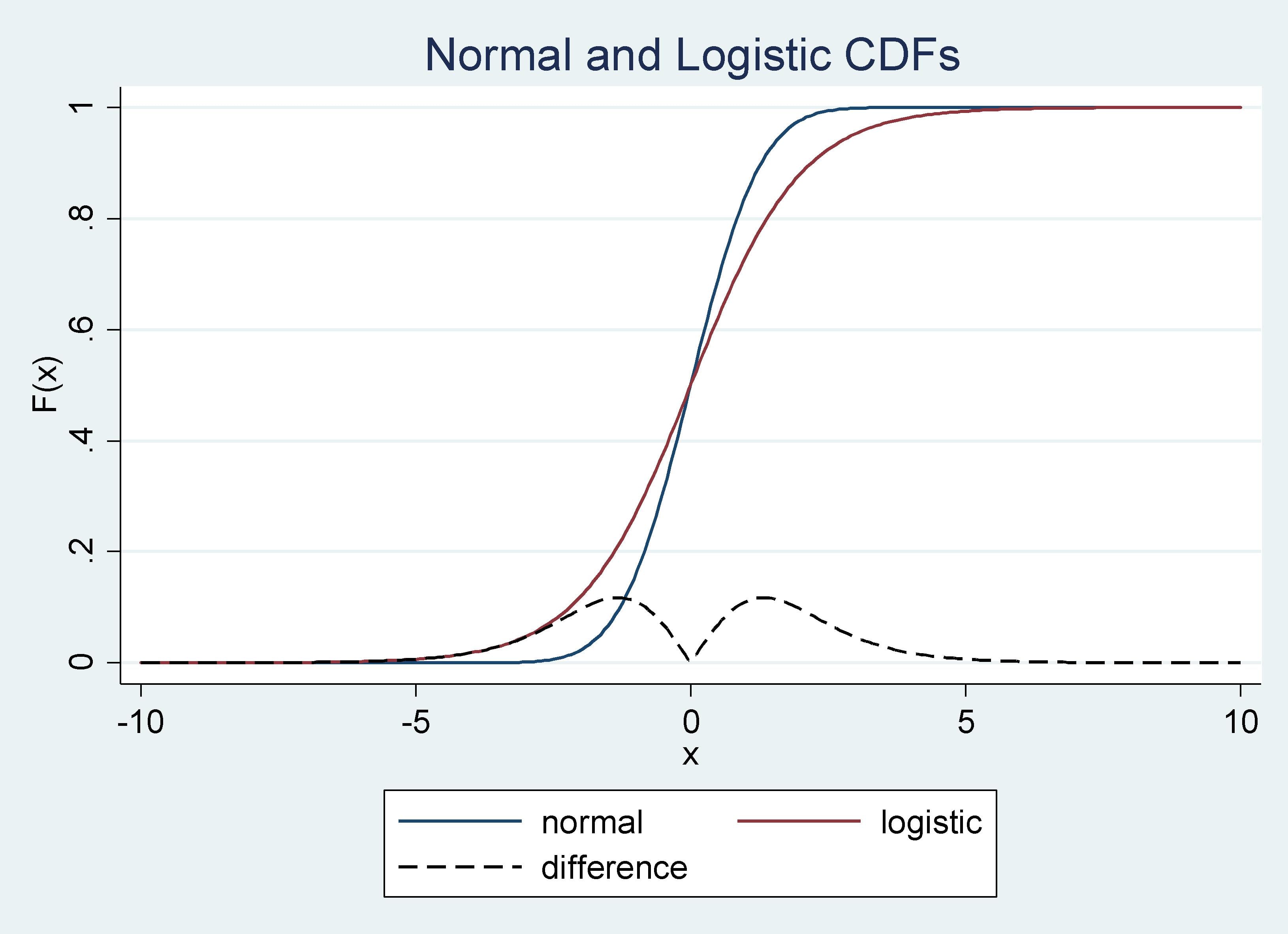
It’s assumed that the unobservable random variable within the probit mannequin and logit mannequin comes from a regular regular and logistic distribution, respectively. The cumulative distribution capabilities (CDFs) in these two circumstances are shut to one another, particularly across the imply. Subsequently, estimators beneath these two units of assumptions produce related outcomes. As an example these arguments, we will plot the 2 CDFs and their variations as follows:
Graph 1: Regular and Logistic CDF’s and their Distinction
The distinction between the CDFs approaches zero as you get nearer to the imply, from the suitable or from the left, and it’s all the time smaller than .15.
Simulation design
Under is the code I used to generate the info for my simulations. Within the first half, traces 4 to 12, I generate consequence variables that fulfill the assumptions of the probit mannequin, y1, and the logit mannequin, y2. Within the second half, traces 13 to 16, I compute the marginal results for the logit and probit fashions. I’ve a steady and a discrete covariate. For the discrete covariate, the marginal impact is a remedy impact. Within the third half, traces 17 to 25, I compute the marginal results evaluated on the means. I’ll use these estimates later to compute approximations to the true values of the results.
program outline mkdata
        syntax, [n(integer 1000)]
        clear
        quietly set obs `n'
        // 1. Producing information from probit, logit, and misspecified
        generate x1    = rnormal()
        generate x2    = rbeta(2,4)>.5
        generate e1    = rnormal()
        generate u     = runiform()
        generate e2    = ln(u) -ln(1-u)
        generate xb    = .5*(1 -x1 + x2)
        generate y1    =  xb + e1 > 0
        generate y2    =  xb + e2 > 0
        // 2. Computing probit & logit marginal and remedy results
        generate m1    = normalden(xb)*(-.5)
        generate m2    = regular(1 -.5*x1 ) - regular(.5 -.5*x1)
        generate m1l   = exp(xb)*(-.5)/(1+exp(xb))^2
        generate m2l   = exp(1 -.5*x1)/(1+ exp(1 -.5*x1 )) - ///
                         exp(.5 -.5*x1)/(1+ exp(.5 -.5*x1 ))
        // 3. Computing probit & logit marginal and remedy results at means
        quietly imply x1 x2
        matrix A         = r(desk)
        scalar a         = .5 -.5*A[1,1] + .5*A[1,2]
        scalar b1        =  1 -.5*A[1,1]
        scalar b0        = .5 -.5*A[1,1]
        generate mean1   = normalden(a)*(-.5)
        generate mean2   = regular(b1) - regular(b0)
        generate mean1l  = exp(a)*(-.5)/(1+exp(a))^2
        generate mean2l  = exp(b1)/(1+ exp(b1)) - exp(b0)/(1+ exp(b0))
finish
I approximate the true marginal results utilizing a pattern of 20 million observations. It is a cheap technique on this case. For instance, take the typical marginal impact for a steady covariate, (x_{okay}), within the case of the probit mannequin:
[begin{equation*}
frac{1}{N}sum_{i=1}^N phileft(x_{i}mathbb{beta}right)beta_{k}
end{equation*}]
The expression above is an approximation to (Eleft(phileft(x_{i}mathbb{beta}proper)beta_{okay}proper)). To acquire this anticipated worth, we would want to combine over the distribution of all of the covariates. This isn’t sensible and would restrict my selection of covariates. As an alternative, I draw a pattern of 20 million observations, compute (frac{1}{N}sum_{i=1}^N phileft(x_{i}mathbb{beta}proper)beta_{okay}), and take it to be the true worth. I observe the identical logic for the opposite marginal results.
Under is the code I take advantage of to compute the approximate true marginal results. I draw the 20 million observations, then I compute the averages that I’m going to make use of in my simulation, and I create locals for every approximate true worth.
. mkdata, n(20000000)

. native values "m1 m2 m1l m2l mean1 mean2 mean1l mean2l"

. native means  "mx1 mx2 mx1l mx2l meanx1 meanx2 meanx1l meanx2l"

. native n : phrase depend `values'

. forvalues i= 1/`n' {
  2.         native a: phrase `i' of `values'
  3.         native b: phrase `i' of `means'
  4.         sum `a', meanonly
  5.         native `b' = r(imply)
  6. }
Now I’m able to run all of the simulations that I used to supply the leads to the earlier part. The code that I used for the simulations for the ATE and the AME when the true DGP is a probit is given by
. postfile mprobit y1p y1p_r y1l y1l_r y2p y2p_r y2l y2l_r ///
>                 utilizing simsmprobit, substitute

. forvalues i=1/4000 {
  2.         quietly {
  3.                 mkdata, n(10000)
  4.                 probit y1 x1 i.x2, vce(strong)
  5.                 margins, dydx(*) atmeans put up
  6.                 native y1p = _b[x1]
  7.                 check _b[x1] = `meanx1'
  8.                 native y1p_r   = (r(p)<.05)
  9.                 native y2p = _b[1.x2]
 10.                 check _b[1.x2] = `meanx2'
 11.                 native y2p_r   = (r(p)<.05)
 12.                 logit  y1 x1 i.x2, vce(strong)
 13.                 margins, dydx(*) atmeans put up
 14.                 native y1l = _b[x1]
 15.                 check _b[x1] = `meanx1'
 16.                 native y1l_r   = (r(p)<.05)
 17.                 native y2l = _b[1.x2]
 18.                 check _b[1.x2] = `meanx2'
 19.                 native y2l_r   = (r(p)<.05)
 20.                 put up mprobit (`y1p') (`y1p_r') (`y1l') (`y1l_r') ///
>                            (`y2p') (`y2p_r') (`y2l') (`y2l_r')
 21.         }
 22. }
. use simsprobit
. summarize

    Variable |        Obs        Imply    Std. Dev.       Min        Max
-------------+---------------------------------------------------------
         y1p |      4,000   -.1536812    .0038952  -.1697037  -.1396532
       y1p_r |      4,000         .05    .2179722          0          1
         y1l |      4,000   -.1536778    .0039179  -.1692524  -.1396366
       y1l_r |      4,000      .05175    .2215496          0          1
         y2p |      4,000     .141708    .0097155   .1111133   .1800973
-------------+---------------------------------------------------------
       y2p_r |      4,000       .0495    .2169367          0          1
         y2l |      4,000    .1416983    .0097459   .1102069   .1789895
       y2l_r |      4,000        .049     .215895          0          1
For the leads to the case of the MEM and the TEM when the true DGP is a probit, I take advantage of margins with the choice atmeans. The opposite circumstances are related. I take advantage of strong normal error for all computations to account for the truth that my chance mannequin is an approximation to the true chance, and I take advantage of the choice vce(unconditional) to account for the truth that I’m utilizing two-step M-estimation. See Wooldridge (2010) for extra particulars on two-step M-estimation.
You may obtain the code used to supply the outcomes by clicking this hyperlink: pvsl.do
Concluding remarks
I offered simulation proof that illustrates that the variations between utilizing estimates of results after probit or logit is negligible. The rationale lies within the principle of quasilikelihood and, particularly, in that the cumulative distribution capabilities of the probit and logit fashions are related, particularly across the imply.
References
White, H. 1996. Estimation, Inference, and Specification Evaluation>. Cambridge: Cambridge College Press.
Wooldridge, J. M. 2010. Econometric Evaluation of Cross Part and Panel Knowledge. 2nd ed. Cambridge, Massachusetts: MIT Press.