

Autoregressive (AR) and moving-average (MA) fashions are mixed to acquire ARMA fashions. The parameters of an ARMA mannequin are usually estimated by maximizing a chance operate assuming independently and identically distributed Gaussian errors. It is a reasonably strict assumption. If the underlying distribution of the error is nonnormal, does most chance estimation nonetheless work? The quick reply is sure beneath sure regularity circumstances and the estimator is named the quasi-maximum chance estimator (QMLE) (White 1982).
On this put up, I exploit Monte Carlo Simulations (MCS) to confirm that the QMLE of a stationary and invertible ARMA mannequin is constant and asymptotically regular. See Yao and Brockwell (2006) for a proper proof. For an outline of performing MCS in Stata, discuss with Monte Carlo simulations utilizing Stata. Additionally see A simulation-based clarification of consistency and asymptotic normality for a dialogue of performing such an train in Stata.
Simulation
Let’s start by simulating from a stationary and invertible ARMA(1,1) course of:
[
y_t = 0.8 y_{t-1} + epsilon_t + 0.5 epsilon_{t-1}
]
I assume a demeaned (chi^2(1)) distribution for (epsilon_t). The next code implements an MCS for the parameters of an ARMA(1,1) course of with demeaned chi-squared improvements. At every repetition, I’ll draw from the method, estimate the parameters of the method, and carry out Wald checks with null hypotheses that correspond to the true parameter values.
. clear all

. set seed 2016

. native MC = 5000

. native T = 100

. quietly postfile armasim ar_t100 ma_t100 rr_ar_t100 rr_ma_t100 utilizing t100,
> exchange

. forvalues i=1/`MC' {
  2.         quietly drop _all
  3.         native obs = `T' + 100
  4.         quietly set obs `obs'
  5.         quietly generate time = _n
  6.         quietly tsset time
  7. /*Generate information*/
.         quietly generate eps = rchi2(1)-1
  8.         quietly generate y = rnormal(0,1) in 1
  9.         quietly exchange y = 0.8*l.y + eps + 0.5*l.eps in 2/l
 10.         quietly drop in 1/100
 11. /*Estimate*/
.         quietly arima y, ar(1) ma(1) nocons vce(sturdy)
 12.         quietly take a look at _b[ARMA:l.ar]=0.8
 13.         native r_ar = (r(p)<0.05)
 14.         quietly take a look at _b[ARMA:l.ma]=0.5
 15.         native r_ma = (r(p)<0.05)
 16.         put up armasim (_b[ARMA:l.ar]) (_b[ARMA:l.ma]) (`r_ar') (`r_ma')
 17. }

. postclose armasim
Traces 1–2 clear Stata and set the seed of the random quantity generator. Traces 3–4 assign the variety of Monte Carlo repetitions and the pattern measurement to native macros MC and T, respectively. Right here I’ll carry out 5,000 Monte Carlo repetitions with a pattern measurement of 100.
In line 5, I exploit postfile to create a spot in reminiscence referred to as armasim to retailer simulation outcomes. We are going to retailer the AR and MA estimates of the ARMA(1,1) mannequin from every Monte Carlo repetition. The outcomes of the Wald checks for the AR and MA parameters will even be saved. These binary variables maintain the worth 1 if the null speculation is rejected on the 5% stage. Every variable is suffixed with the pattern measurement, and can be saved within the dataset t100.
I exploit forvalues to carry out the Monte Carlo repetitions. Every time by the forvalues loop, I begin by dropping all variables and setting the variety of observations to the pattern measurement plus 100. These first 100 observations can be discarded as burn-in. I then generate a time variable and declare it as time-series information.
Subsequent, I generate information from an ARMA(1,1) course of. First, I draw demeaned (chi^2(1)) improvements and retailer them within the variable eps. I retailer the noticed collection in y. The burn-in observations are then dropped.
I estimate the parameters of the ARMA(1,1) mannequin utilizing the arima command, which on this case needs to be interpreted as a QMLE. Notice that I specify nocons to suppress the fixed time period. I exploit vce(sturdy) to request customary errors sturdy to misspecification as a result of the default customary errors are primarily based on a traditional distribution and are invalid on this case. I take a look at whether or not the parameters are equal to their true values and use the put up command to retailer the estimates together with the rejection charges of the Wald checks in armasim.
After the forvalues loop, I shut armasim in reminiscence utilizing postclose. This protects all of the estimates within the dataset t100.
I’ve demonstrated the best way to carry out a Monte Carlo simulation with 5,000 repetitions of an ARMA(1,1) course of with a pattern measurement of 100. I repeat the identical experiment for a pattern measurement of 1,000 and 10,000 and retailer the estimates within the datasets t1000 and t10000, respectively. The code is supplied within the Appendix.
Now, I consider the outcomes of the simulations for the QMLE of the AR parameter. The identical strategies can be utilized to judge the estimator for the MA parameter.
Consistency
A constant estimator will get arbitrarily shut in likelihood to the true worth as you enhance the pattern measurement. I’ll assess the consistency of the QMLE for the AR parameter by evaluating the outcomes of our three simulations.
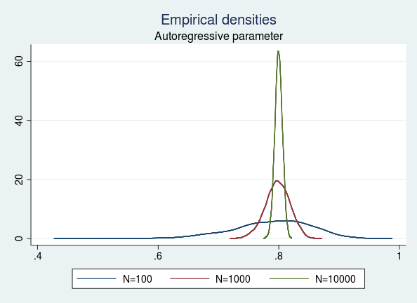
I load the t100 information in reminiscence and merge with the t1000 and t10000 datasets utilizing the merge command. Then I plot the empirical densities of the estimated AR parameter for the three pattern sizes.
. use t100, clear

. quietly merge 1:1 _n utilizing t1000

. drop _merge

. quietly merge 1:1 _n utilizing t10000

. drop _merge

. kdensity ar_t100, n(5000) generate(x_100 f_100) kernel(gaussian) nograph

. label variable f_100 "N=100"

. kdensity ar_t1000, n(5000) generate(x_1000 f_1000) kernel(gaussian) nograph

. label variable f_1000 "N=1000"

. kdensity ar_t10000, n(5000) generate(x_10000 f_10000) kernel(gaussian)
> nograph

. label variable f_10000 "N=10000"

. graph twoway (line f_100 x_100) (line f_1000 x_1000) (line f_10000 x_10000),
> legend(rows(1)) title("Empirical densities") subtitle("Autoregressive paramet
> er")
The empirical distribution for the estimated AR parameter is tighter across the true worth of 0.8 for a pattern measurement of 10,000 than that for a pattern of measurement 100. The determine implies that as we preserve rising the pattern measurement to (infty), the AR estimate converges to the true worth with likelihood 1. This means that the QMLE is constant.
Asymptotic normality
If (hat{theta}_{textrm{QMLE}}) is a constant estimator of the true worth (theta), then (sqrt{T}(hat{theta}_{textrm{QMLE}}-theta)) converges in distribution to (N(0,V)) as (T) approaches (infty) (White 1982). Assuming I’ve an infinite variety of observations, the sturdy variance estimator offers a very good approximation to the true variance. On this case, I get hold of the “true” variance for the recentered and rescaled AR parameter to be 0.42 by utilizing the sturdy variance estimator on a 10-million statement pattern.
Let us take a look at the recentered and rescaled model of the empirical distributions of the AR parameters obtained for various pattern sizes. I plot all of the empirical distributions together with the “true” N(0,0.42) distribution for comparability.
. generate double ar_t100n = sqrt(100)*(ar_t100 - 0.8)

. generate double ar_t1000n = sqrt(1000)*(ar_t1000 - 0.8)

. generate double ar_t10000n = sqrt(10000)*(ar_t10000 - 0.8)

. kdensity ar_t100n, n(5000) generate(x_100n f_100n) kernel(gaussian) nograph

. label variable f_100n "N=100"

. kdensity ar_t1000n, n(5000) generate(x_1000n f_1000n) kernel(gaussian)
> nograph

. label variable f_1000n "N=1000"

. kdensity ar_t10000n, n(5000) generate(x_10000n f_10000n) kernel(gaussian)
> nograph

. label variable f_10000n "N=10000"

twoway (line f_100n x_100n) (line f_1000n x_1000n) (line f_10000n x_10000n) (4
> operate normalden(x, sqrt(0.42)), vary(-4 4)), legend( label(4 "Regular(0, 0
> .42)") cols(3)) title("Empirical densities") subtitle("Recentered and rescale
> d estimator and a N(0,0.42)")
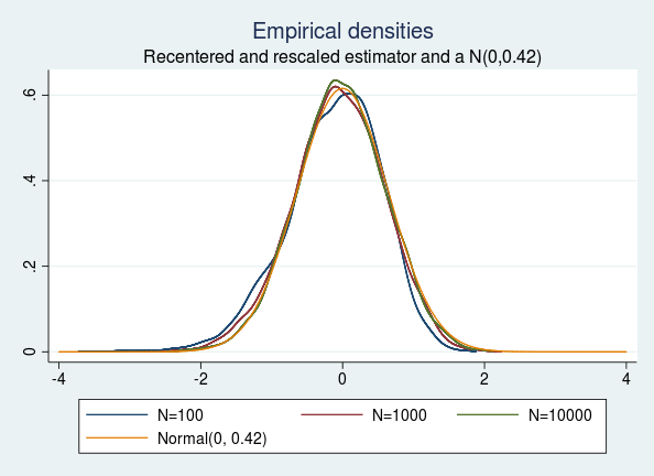
We see that the empirical densities of the recentered and rescaled estimators are indistinguishable from the density of a traditional distribution with imply 0 and variance 0.42, as predicted by the speculation.
Estimating rejection charges
I additionally assess the estimated customary error and asymptotic normality of the QMLE by checking the rejection charges. The Wald checks rely upon the asymptotic normality of the estimate and a constant estimate of the usual error. Summarizing the imply of the rejection charges of the estimated ARMA(1,1) for all pattern sizes yields the next desk.
. imply rr_ar* rr_ma*

Imply estimation                   Variety of obs   =      5,000

--------------------------------------------------------------
             |       Imply   Std. Err.     [95% Conf. Interval]
-------------+------------------------------------------------
  rr_ar_t100 |       .069   .0035847      .0619723    .0760277
 rr_ar_t1000 |      .0578   .0033006      .0513294    .0642706
rr_ar_t10000 |      .0462    .002969      .0403795    .0520205
  rr_ma_t100 |      .0982   .0042089      .0899487    .1064513
 rr_ma_t1000 |       .056   .0032519      .0496248    .0623752
rr_ma_t10000 |       .048   .0030234      .0420728    .0539272
--------------------------------------------------------------
The rejection charges for the AR and MA parameters are massive in contrast with the nominal measurement of 5% for a pattern measurement of 100. As I enhance the pattern measurement, the rejection price will get nearer to the nominal measurement. This means that the sturdy variance estimator yields a very good protection of the Wald take a look at in massive samples.
Conclusion
I used MCS to confirm the consistency and asymptotic normality of the QMLE of an ARMA(1,1) mannequin. I estimated the rejection charges for the AR and MA parameters utilizing MCS and likewise verified that the sturdy variance estimator constantly estimates the true variance of the QMLE in massive samples.
Appendix
MCS for a pattern measurement of 1,000
. native T = 1000

. quietly postfile armasim ar_t1000 ma_t1000 rr_ar_t1000 rr_ma_t1000 utilizing
> t1000, exchange

. forvalues i=1/`MC' {
  2.         quietly drop _all
  3.         native obs = `T' + 100
  4.         quietly set obs `obs'
  5.         quietly generate time = _n
  6.         quietly tsset time
  7. /*Generate information*/
.         quietly generate eps = rchi2(1)-1
  8.         quietly generate y = rnormal(0,1) in 1
  9.         quietly exchange y = 0.8*l.y + eps + 0.5*l.eps in 2/l
 10.         quietly drop in 1/100
 11. /*Estimate*/
.         quietly arima y, ar(1) ma(1) nocons vce(sturdy)
 12.         quietly take a look at _b[ARMA:l.ar]=0.8
 13.         native r_ar = (r(p)<0.05)
 14.         quietly take a look at _b[ARMA:l.ma]=0.5
 15.         native r_ma = (r(p)<0.05)
 16.         put up armasim (_b[ARMA:l.ar]) (_b[ARMA:l.ma]) (`r_ar') (`r_ma')
 17. }

. postclose armasim
MCS for a pattern measurement of 10,000
. native T = 10000

. quietly postfile armasim ar_t10000 ma_t10000 rr_ar_t10000 rr_ma_t10000 utilizing
> t10000, exchange

. forvalues i=1/`MC' {
  2.         quietly drop _all
  3.         native obs = `T' + 100
  4.         quietly set obs `obs'
  5.         quietly generate time = _n
  6.         quietly tsset time
  7. /*Generate information*/
.         quietly generate eps = rchi2(1)-1
  8.         quietly generate y = rnormal(0,1) in 1
  9.         quietly exchange y = 0.8*l.y + eps + 0.5*l.eps in 2/l
 10.         quietly drop in 1/100
 11. /*Estimate*/
.         quietly arima y, ar(1) ma(1) nocons vce(sturdy)
 12.         quietly take a look at _b[ARMA:l.ar]=0.8
 13.         native r_ar = (r(p)<0.05)
 14.         quietly take a look at _b[ARMA:l.ma]=0.5
 15.         native r_ma = (r(p)<0.05)
 16.         put up armasim (_b[ARMA:l.ar]) (_b[ARMA:l.ma]) (`r_ar') (`r_ma')
 17. }

. postclose armasim
References
White, H. L., Jr. 1982. Most chance estimation of misspecified fashions. Econometrica 50: 1–25.
Yao, Q., and P. J. Brockwell. 2006. Gaussian most chance estimation for ARMA fashions I: time collection. Journal of Time Collection Evaluation 27: 857–875.