

(newcommand{Eb}{{bf E}}
newcommand{xb}{{bf x}}
newcommand{betab}{boldsymbol{beta}})Variations in conditional chances and ratios of odds are two widespread measures of the impact of a covariate in binary-outcome fashions. I present how these measures differ by way of conditional-on-covariate results versus population-parameter results.
Distinction in commencement chances
I’ve simulated information on whether or not a scholar graduates in 4 years (graduate) for every of 1,000 college students that entered an imaginary college in the identical 12 months. Earlier than beginning their first 12 months, every scholar took a brief course that taught research strategies and new materials; iexam data every scholar’s grade on the ultimate for this course. I’m within the impact of the mathematics and verbal SAT rating sat on the chance that graduate=1 once I additionally situation on high-school grade-point common hgpa and iexam. I embody an interplay time period it=iexam/(hgpa^2) within the regression to permit for the chance that iexam has a smaller impact for college kids with the next hgpa. You may obtain the info by clicking on effectsb.dta.
Under I estimate the parameters of a logistic mannequin that specifies the chance of commencement conditional on values of hgpa, sat, and iexam. (From right here on, commencement chance is brief for four-year commencement chance.)
Instance 1: Logistic mannequin for commencement chance situation on hgpa, sat, and iexam
. logit grad hgpa sat iexam it

Iteration 0:   log chance = -692.80914
Iteration 1:   log chance = -404.97166
Iteration 2:   log chance = -404.75089
Iteration 3:   log chance = -404.75078
Iteration 4:   log chance = -404.75078

Logistic regression                             Variety of obs     =      1,000
                                                LR chi2(4)        =     576.12
                                                Prob > chi2       =     0.0000
Log chance = -404.75078                     Pseudo R2         =     0.4158

------------------------------------------------------------------------------
        grad |      Coef.   Std. Err.      z    P>|z|     [95% Conf. Interval]
-------------+----------------------------------------------------------------
        hgpa |   2.347051   .3975215     5.90   0.000     1.567923    3.126178
         sat |   1.790551   .1353122    13.23   0.000     1.525344    2.055758
       iexam |   1.447134   .1322484    10.94   0.000     1.187932    1.706336
          it |   1.713286   .7261668     2.36   0.018     .2900249    3.136546
       _cons |  -46.82946   3.168635   -14.78   0.000    -53.03987   -40.61905
------------------------------------------------------------------------------
The estimates suggest that
start{align*}
widehat{bf Pr}[{bf graduate=1}&| {bf hgpa}, {bf sat}, {bf iexam}]
& = {bf F}left[
2.35{bf hgpa} + 1.79 {bf sat} + 1.45 {bf iexam}right.
&quad left. + 1.71 {bf iexam}/{(bf hgpa^2)} – 46.83right]
finish{align*}
the place ({bf F}(xbbetab)=exp(xbbetab)/[1+exp(xbbetab)]) is the logistic distribution and (widehat{bf Pr}[{bf graduate=1}| {bf hgpa}, {bf sat}, {bf iexam}]) denotes the estimated conditional chance operate.
Suppose that I’m a researcher who needs to know the impact of getting a 1400 as a substitute of a 1300 on the SAT on the conditional commencement chance. As a result of sat is measured in a whole bunch of factors, the impact is estimated to be
start{align*}
widehat{bf Pr}&[{bf graduate=1}|{bf sat}=14, {bf hgpa}, {bf iexam}]
&hspace{1cm}
-widehat{bf Pr}[{bf graduate=1}|{bf sat}=13, {bf hgpa}, {bf iexam}]
& = {bf F}left[
2.35{bf hgpa} + 1.79 (14) + 1.45 {bf iexam}
+ 1.71 {bf iexam}/{(bf hgpa^2)} – 46.83right]
& hspace{1cm} –
{bf F}left[
2.35{bf hgpa} + 1.79 (13) + 1.45 {bf iexam}
+ 1.71 {bf iexam}/{(bf hgpa^2)} – 46.83right]
finish{align*}
The estimated impact of going from 1300 to 1400 on the SAT varies over the values of hgpa and iexam, as a result of ({bf F}()) is nonlinear.
In instance 2, I take advantage of predictnl to estimate these results for every commentary within the pattern, after which I graph them.
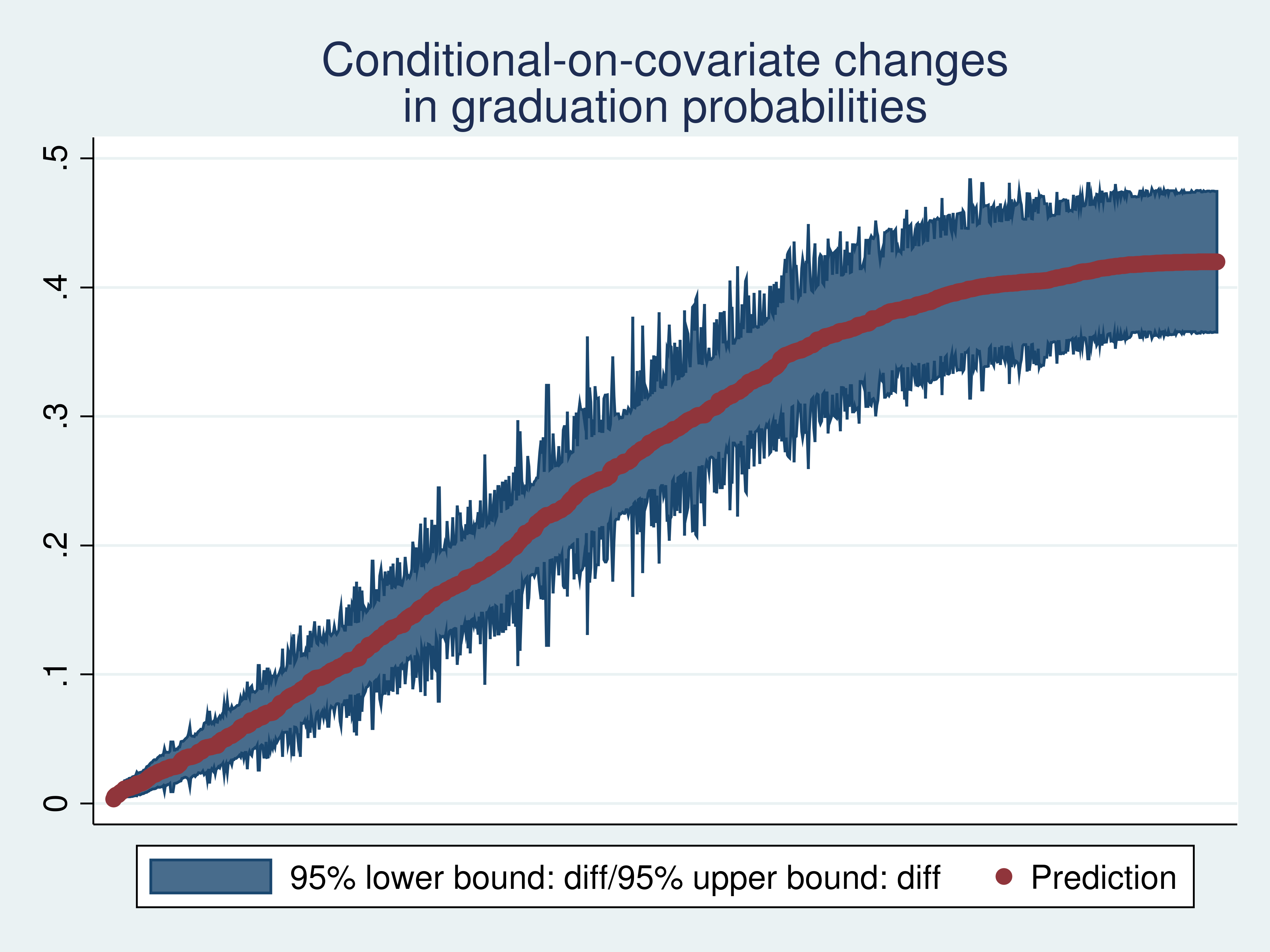
Instance 2: Estimated modifications in commencement chances
. predictnl double diff =
>    logistic( _b[hgpa]*hgpa + _b[sat]*14 + _b[iexam]*iexam + _b[it]*it + _b[_cons])
>  - logistic( _b[hgpa]*hgpa + _b[sat]*13 + _b[iexam]*iexam + _b[it]*it + _b[_cons])
>    , ci(low up)
observe: confidence intervals calculated utilizing Z vital values

. type diff

. generate ob = _n

. twoway (rarea low up ob) (scatter diff ob) , xlabels(none) xtitle("")
>    title("Conditional-on-covariate modifications" "in commencement chances")
I see that the estimated variations in conditional commencement chances attributable to going from 1300 to 1400 on the SAT vary from near 0 to greater than 0.4 over the pattern values of hgpa and iexam.
If I have been a counselor advising particular college students on the idea of their hgpa and iexam values, I might have an interest wherein college students had results close to zero and wherein college students had results higher than, say, 0.3. Methodologically, I might be desirous about results conditional on the covariates hgpa and iexam.
As an alternative, suppose I wish to know “whether or not going from 1300 to 1400 on the SAT issues”, and I’m thus desirous about a single combination measure. In instance 3, I take advantage of margins to estimate the imply of the conditional-on-covariate results.
Instance 3: Estimated imply of conditional modifications in commencement chances
. margins , at(sat=(13 14)) distinction(atcontrast(r._at) nowald)

Contrasts of predictive margins
Mannequin VCE    : OIM

Expression   : Pr(grad), predict()

1._at        : sat             =          13

2._at        : sat             =          14

--------------------------------------------------------------
             |            Delta-method
             |   Distinction   Std. Err.     [95% Conf. Interval]
-------------+------------------------------------------------
         _at |
   (2 vs 1)  |   .2576894   .0143522      .2295597    .2858192
--------------------------------------------------------------
The imply change within the conditional commencement chances attributable to going from 1300 to 1400 on the SAT is estimated to be 0.22. It seems that this imply change is similar because the distinction within the chances which might be solely conditioned on the hypothesized sat values.
start{align*}
Eb&left[
widehat{bf Pr}[{bf graduate=1}|{bf sat}=14, {bf hgpa}, {bf iexam}] proper.
&quad
left. -widehat{bf Pr}[{bf graduate=1}|{bf sat}=13, {bf hgpa}, {bf iexam}]
proper]
& =
widehat{bf Pr}[{bf graduate=1}|{bf sat}=14]
–
widehat{bf Pr}[{bf graduate=1}|{bf sat}=13]
finish{align*}
The imply of the modifications within the conditional chances is a change in marginal chances. ((widehat{bf Pr}[{bf graduate=1}|{bf sat}=14]) and (widehat{bf Pr}[{bf graduate=1}|{bf sat}=13]) are conditional on the hypothesized sat values of curiosity and are marginal over hgpa and iexam.) The distinction within the chances that situation solely the values that outline the “remedy” values is likely one of the inhabitants parameters {that a} potential-outcome strategy would specify to be of curiosity.
Odds ratios
The percentages of an occasion specifies how doubtless it’s to happen, with larger values implying that the occasion is extra doubtless. An odds ratio is the ratio of the chances of an occasion in a single state of affairs to the chances of the identical occasion beneath a distinct state of affairs. For instance, I could be within the ratio of the commencement odds when a scholar has an SAT of 1400 to the commencement odds when a scholar has an SAT of 1300. A worth higher than 1 implies that going from 1300 to 1400 has raised the commencement odds. A worth lower than 1 implies that going from 1300 to 1400 has lowered the commencement odds.
As a result of we used a logistic mannequin for the conditional chance, the ratio of the chances of commencement conditional on sat=14, hgpa, and iexam to the chances of commencement conditional on sat=13, hgpa, and iexam is exp(_b[sat]), whose estimate we will acquire from
logit.
Instance 4: Ratio of conditional-on-covariate commencement odds
. logit , or

Logistic regression                             Variety of obs     =      1,000
                                                LR chi2(4)        =     576.12
                                                Prob > chi2       =     0.0000
Log chance = -404.75078                     Pseudo R2         =     0.4158

------------------------------------------------------------------------------
        grad | Odds Ratio   Std. Err.      z    P>|z|     [95% Conf. Interval]
-------------+----------------------------------------------------------------
        hgpa |   10.45469   4.155964     5.90   0.000     4.796674    22.78673
         sat |   5.992756   .8108931    13.23   0.000     4.596726    7.812761
       iexam |   4.250916   .5621767    10.94   0.000     3.280292    5.508743
          it |   5.547158   4.028162     2.36   0.018     1.336461    23.02421
       _cons |   4.59e-21   1.46e-20   -14.78   0.000     9.23e-24    2.29e-18
------------------------------------------------------------------------------
The conditional-on-covariate commencement odds are estimated to be 6 instances larger for a scholar with a 1400 SAT than for a scholar with a 1300 SAT. This interpretation comes from some algebra that exhibits that
start{align*}
{giant frac{
frac{widehat{bf Pr}[{bf graduate=1}|{bf sat}=14, {bf hgpa}, {bf iexam}]}{
1-widehat{bf Pr}[{bf graduate=1}|{bf sat}=14, {bf hgpa}, {bf iexam}]}
}
{
frac{widehat{bf Pr}[{bf graduate=1}|{bf sat}=13, {bf hgpa}, {bf iexam}]}{
1-widehat{bf Pr}[{bf graduate=1}|{bf sat}=13, {bf hgpa}, {bf iexam}]}
}}
=expleft({bf _b[sat]}proper)
finish{align*}
when
start{align*}
&hspace{-.5em}widehat{bf Pr}[{bf graduate=1}|{bf sat}, {bf hgpa}, {bf iexam}]
&hspace{-.5em}= {small frac{
{bf exp(
_b[hgpa] hgpa
+ _b[sat] sat
+ _b[iexam] iexam
+ _b[it] it
+ _b[_cons]
)}
}
{
1 +
{bf exp(
_b[hgpa] hgpa
+ _b[sat] sat
+ _b[iexam] iexam
+ _b[it] it
+ _b[_cons]
)}
}}
finish{align*}
In truth, a extra normal assertion is feasible. exp(_b[sat]) is the ratio of the conditional-on-covariate commencement odds for a scholar getting another unit of sat to the conditional-on-covariate commencement odds for a scholar getting his or her present sat worth.
As an alternative, I wish to spotlight that the logistic useful kind makes this odds ratio a continuing and that the ratio of conditional-on-covariate odds differs from the ratio of odds that situation solely the hypothesized values.
Instance 5 illustrates that the conditional-on-covariate odds ratio doesn’t fluctuate over the covariate patterns within the pattern.
Instance 5: Odds-ratio calculation
. generate sat_orig = sat

. change sat  = 13
(999 actual modifications made)

. predict double pr0
(possibility pr assumed; Pr(grad))

. change sat  = 14
(1,000 actual modifications made)

. predict double pr1
(possibility pr assumed; Pr(grad))

. change sat  = sat_orig
(993 actual modifications made)

. generate orc = (pr1/(1-pr1))/(pr0/(1-pr0))

. summarize orc

    Variable |        Obs        Imply    Std. Dev.       Min        Max
-------------+---------------------------------------------------------
         orc |      1,000    5.992756           0   5.992756   5.992756
That the usual deviation is 0 highlights that the values are fixed.
The ratio of the commencement odds that situation solely on the hypothesized sat values differs from the imply of the ratios of commencement odds that situation on the hypothesized sat values and on hgpa and iexam. In distinction, the distinction within the commencement chances that situation solely on the hypothesized sat values is similar because the imply of the variations in commencement chances that situation on the hypothesized sat values and on hgpa and iexam.
Instance 6 estimates the ratio of commencement odds that situation solely on the hypothesized sat values.
Instance 6: Odds ratio that situations solely on hypothesized sat values
. margins , at(sat=(13 14)) submit

Predictive margins                              Variety of obs     =      1,000
Mannequin VCE    : OIM

Expression   : Pr(grad), predict()

1._at        : sat             =          13

2._at        : sat             =          14

------------------------------------------------------------------------------
             |            Delta-method
             |     Margin   Std. Err.      z    P>|z|     [95% Conf. Interval]
-------------+----------------------------------------------------------------
         _at |
          1  |   .2430499    .018038    13.47   0.000     .2076961    .2784036
          2  |   .5007393   .0133553    37.49   0.000     .4745634    .5269152
------------------------------------------------------------------------------

. nlcom (_b[2._at]/(1-_b[2._at]))/(_b[1._at]/(1-_b[1._at]))

       _nl_1:  (_b[2._at]/(1-_b[2._at]))/(_b[1._at]/(1-_b[1._at]))

------------------------------------------------------------------------------
             |      Coef.   Std. Err.      z    P>|z|     [95% Conf. Interval]
-------------+----------------------------------------------------------------
       _nl_1 |   3.123606   .2418127    12.92   0.000     2.649661     3.59755
------------------------------------------------------------------------------
Mathematically, this estimate implies that
start{align*}
giant{frac{
frac{widehat{bf Pr}[{bf graduate=1}|{bf sat}=14 ]}{
1-widehat{bf Pr}[{bf graduate=1}|{bf sat}=14 ]}
}
{
frac{widehat{bf Pr}[{bf graduate=1}|{bf sat}=13 ]}{
1-widehat{bf Pr}[{bf graduate=1}|{bf sat}=13 ]}
}}
= 3.12
finish{align*}
The Delta-method commonplace error gives inference for the scholar on this pattern versus an unconditional commonplace error that gives inference for repeated pattern from the inhabitants. (See Medical doctors versus coverage analysts: Estimating the impact of curiosity for an instance of find out how to acquire an unconditional commonplace error.)
The imply of a nonlinear operate differs from a nonlinear operate evaluated on the imply. Thus, the imply of conditional-on-covariate odds ratios differs from the chances ratio computed utilizing technique of conditional-on-covariate chances.
Which odds ratio is of curiosity is determined by what you wish to know. The conditional-on-covariate odds ratio is of curiosity when conditional-on-covariate comparisons are the purpose, as is for the counselor mentioned above. The ratio of the chances that situation solely on hypothesized sat values is the inhabitants parameter {that a} potential-outcome strategy would specify to be of curiosity.
Finished and undone
Along with discussing variations between conditional-on-covariate inference and inhabitants inference, I highlighted a distinction between generally used impact measures. The imply of variations in conditional-on-covariate chances is similar as a potential-outcome inhabitants parameter. In distinction, the imply of conditional-on-covariate odds ratios differs from the potential-outcome inhabitants parameter.