

When becoming nearly any mannequin, we could also be considering investigating whether or not parameters differ throughout teams equivalent to time intervals, age teams, gender, or faculty attended. In different phrases, we could want to carry out assessments of moderation when the moderator variable is categorical. For regression fashions, this may be so simple as together with group indicators within the mannequin and interacting them with different predictors.
We naturally have hypotheses relating to variations in parameters throughout teams when becoming structural equation fashions as nicely. When these fashions contain latent variables and the corresponding noticed measurements, we are able to take a look at whether or not these measurements are invariant throughout teams. Analysis of measurement invariance sometimes entails a sequence of assessments for equality of measurement coefficients (issue loadings), equality of intercepts, and equality of error variances throughout teams.
On this publish, I reveal how one can use the sem command’s group() and ginvariant() choices in addition to the postestimation command estat ginvariant to simply carry out assessments of measurement invariance.
Measurement invariance instance
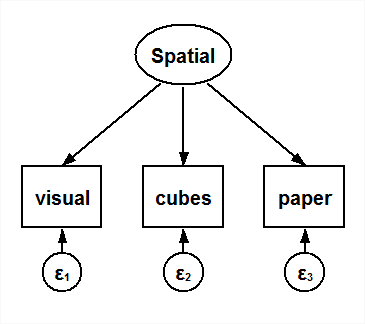
I take advantage of knowledge from Holzinger and Swineford (1939), which information college students’ scores on quite a few exams designed to measure various kinds of talents. The scholars on this dataset got here from two totally different colleges, the Pasteur faculty and the Grant-White faculty, and I need to take a look at for variations throughout colleges. Right here I give attention to three exams that have been meant to measure spatial talents. I’ll match the confirmatory issue mannequin akin to the next path diagram and carry out a sequence of assessments for measurement invariance. Though this instance makes use of the sem command, I may have equivalently drawn this diagram within the Builder and chosen group evaluation to suit all of the fashions mentioned beneath.
To start, I match a mannequin with all parameters estimated individually throughout teams. There are numerous methods to set the required figuring out constraints that present a scale and placement for the latent variable. Right here I set the imply of the Spatial latent variable to 0 and the variance to 1 in each teams.
. sem (Spatial -> visible cubes paper),
> variance(Spatial@1) imply(Spatial@0) ginvariant(none) group(faculty)

Endogenous variables

Measurement:  visible cubes paper

Exogenous variables

Latent:       Spatial

Becoming goal mannequin:

Iteration 0:   log chance = -2603.5782
Iteration 1:   log chance = -2603.5782

Structural equation mannequin                       Variety of obs     =        301
Grouping variable  = faculty                     Variety of teams  =          2
Estimation methodology  = ml
Log chance     = -2603.5782

 ( 1)  [var(Spatial)]1bn.faculty = 1
 ( 2)  [mean(Spatial)]1bn.faculty = 0
 ( 3)  [var(Spatial)]2.faculty = 1
 ( 4)  [mean(Spatial)]2.faculty = 0
-------------------------------------------------------------------------------
              |                 OIM
              |      Coef.   Std. Err.      z    P>|z|     [95% Conf. Interval]
--------------+----------------------------------------------------------------
Measurement   |
  visible <-   |
      Spatial |
     Pasteur  |   4.264065   .8600633     4.96   0.000     2.578372    5.949759
  Grant-Wh~e  |    5.49895   1.190435     4.62   0.000     3.165739     7.83216
        _cons |
     Pasteur  |   29.64744   .5674293    52.25   0.000     28.53529    30.75958
  Grant-Wh~e  |   29.57931   .5721785    51.70   0.000     28.45786    30.70076
  ------------+----------------------------------------------------------------
  cubes <-    |
      Spatial |
     Pasteur  |    2.26321   .5214501     4.34   0.000     1.241187    3.285234
  Grant-Wh~e  |   1.808245   .5031516     3.59   0.000     .8220861    2.794404
        _cons |
     Pasteur  |    23.9359   .3927222    60.95   0.000     23.16618    24.70562
  Grant-Wh~e  |       24.8   .3678649    67.42   0.000       24.079      25.521
  ------------+----------------------------------------------------------------
  paper <-    |
      Spatial |
     Pasteur  |   1.695466   .3429472     4.94   0.000     1.023302     2.36763
  Grant-Wh~e  |   1.311235   .3413206     3.84   0.000     .6422592    1.980211
        _cons |
     Pasteur  |   14.16026    .227089    62.36   0.000     13.71517    14.60534
  Grant-Wh~e  |   14.30345   .2335324    61.25   0.000     13.84573    14.76116
--------------+----------------------------------------------------------------
 imply(Spatial)|
          [*] |          0  (constrained)
--------------+----------------------------------------------------------------
 var(e.visible)|
     Pasteur  |   32.04601   6.912718                       20.9971    48.90898
 Grant-White  |   17.23285   12.18676                      4.309258    68.91467
  var(e.cubes)|
     Pasteur  |   18.93787   2.710244                      14.30585    25.06967
 Grant-White  |   16.35232   2.318816                      12.38443    21.59149
  var(e.paper)|
     Pasteur  |   5.170226    1.09911                      3.408453    7.842631
 Grant-White  |   6.188581   .9975804                      4.512114    8.487938
  var(Spatial)|
          [*] |          1  (constrained)
-------------------------------------------------------------------------------
Observe: [*] identifies parameter estimates constrained to be equal throughout teams.
LR take a look at of mannequin vs. saturated: chi2(0)   =      0.00, Prob > chi2 =      .
Glancing by this output, we see that most of the parameter estimates are very related for the 2 colleges. The estat ginvariant command gives assessments of invariance throughout teams.
. estat ginvariant, showpclass(mcoef) class

Assessments for group invariance of parameters

------------------------------------------------------------------------------
             |            Wald Check                       Rating Check
             |      chi2         df    p>chi2       chi2          df    p>chi2
-------------+----------------------------------------------------------------
Measurement  |
  visible <-  |
     Spatial |     0.707          1    0.4004          .           .         .
  -----------+----------------------------------------------------------------
  cubes <-   |
     Spatial |     0.394          1    0.5301          .           .         .
  -----------+----------------------------------------------------------------
  paper <-   |
     Spatial |     0.631          1    0.4271          .           .         .
------------------------------------------------------------------------------

Joint assessments for every parameter class

------------------------------------------------------------------------------
             |            Wald Check                       Rating Check
             |      chi2         df    p>chi2       chi2          df    p>chi2
-------------+----------------------------------------------------------------
       mcoef |     1.097          3    0.7778          .           .         .
------------------------------------------------------------------------------
The showpclass(mcoef) and class choices restricted the outcomes to assessments relating to measurement coefficients and requested a joint take a look at for the speculation that every one measurement coefficients are equal throughout teams. The primary desk within the output stories separate assessments of equality of the measurement coefficients throughout teams. My focus now, nonetheless, is on the joint Wald take a look at proven within the second desk, and we fail to reject the speculation of equality throughout teams for all measurement coefficients.
I now embrace the ginvariant(mcoef) possibility as a way to match a mannequin with the measurement coefficients constrained to be equal throughout teams by typing
. sem (Spatial -> visible cubes paper), variance(Spatial@1) ///
       imply(Spatial@0) ginvariant(mcoef) group(faculty)
after which take a look at whether or not the intercepts will be constrained:
. estat ginvariant, showpclass(mcons) class

Assessments for group invariance of parameters

------------------------------------------------------------------------------
             |            Wald Check                       Rating Check
             |      chi2         df    p>chi2       chi2          df    p>chi2
-------------+----------------------------------------------------------------
Measurement  |
  visible <-  |
       _cons |     0.007          1    0.9326          .           .         .
  -----------+----------------------------------------------------------------
  cubes <-   |
       _cons |     2.580          1    0.1082          .           .         .
  -----------+----------------------------------------------------------------
  paper <-   |
       _cons |     0.193          1    0.6605          .           .         .
------------------------------------------------------------------------------

Joint assessments for every parameter class

------------------------------------------------------------------------------
             |            Wald Check                       Rating Check
             |      chi2         df    p>chi2       chi2          df    p>chi2
-------------+----------------------------------------------------------------
       mcons |     3.011          3    0.3900          .           .         .
------------------------------------------------------------------------------
We fail to reject the null speculation that every one intercepts are equal throughout teams, so I match the mannequin with these equality constraints by specifying the ginvariant(mcoef mcons) possibility.
. sem (Spatial -> visible cubes paper), variance(Spatial@1) ///
      imply(Spatial@0) ginvariant(mcoef mcons) group(faculty)
Then, I take a look at the equality of the error variances.
. estat ginvariant, showpclass(merrvar) class

Assessments for group invariance of parameters

------------------------------------------------------------------------------
             |            Wald Check                       Rating Check
             |      chi2         df    p>chi2       chi2          df    p>chi2
-------------+----------------------------------------------------------------
var(e.visible)|     0.359          1    0.5493          .           .         .
 var(e.cubes)|     1.413          1    0.2345          .           .         .
 var(e.paper)|     0.014          1    0.9052          .           .         .
------------------------------------------------------------------------------

Joint assessments for every parameter class

------------------------------------------------------------------------------
             |            Wald Check                       Rating Check
             |      chi2         df    p>chi2       chi2          df    p>chi2
-------------+----------------------------------------------------------------
     merrvar |     1.857          3    0.6027          .           .         .
------------------------------------------------------------------------------
As soon as once more, we fail to reject the null speculation of invariance throughout teams. I now impose constraints on the coefficients, intercepts, and error variances whereas permitting the imply and variance of the latent variable to vary throughout teams. To do that, I take away the imply(Spatial@0) possibility and exchange the variance(Spatial@1) with variance(1:Spatial@1). With this variation, the imply and variance of Spatial can be set to 0 and 1, respectively, within the first group however estimated freely within the second group.
. sem (Spatial -> visible cubes paper),
> variance(1:Spatial@1) ginvariant(mcoef mcons merrvar) group(faculty)

Endogenous variables

Measurement:  visible cubes paper

Exogenous variables

Latent:       Spatial

Becoming goal mannequin:

Iteration 0:   log chance = -5357.6935  (not concave)
Iteration 1:   log chance = -4792.5814  (not concave)
Iteration 2:   log chance = -4316.3827  (not concave)
Iteration 3:   log chance =  -2769.069  (not concave)
Iteration 4:   log chance = -2662.2605
Iteration 5:   log chance = -2645.7652
Iteration 6:   log chance = -2629.1987
Iteration 7:   log chance =   -2622.83  (not concave)
Iteration 8:   log chance = -2622.3555
Iteration 9:   log chance = -2622.3227
Iteration 10:  log chance = -2621.9007
Iteration 11:  log chance = -2621.8931
Iteration 12:  log chance =  -2621.893

Structural equation mannequin                       Variety of obs     =        301
Grouping variable  = faculty                     Variety of teams  =          2
Estimation methodology  = ml
Log chance     =  -2621.893

 ( 1)  [cubes]1bn.faculty#c.Spatial - [cubes]2.faculty#c.Spatial = 0
 ( 2)  [paper]1bn.faculty#c.Spatial - [paper]2.faculty#c.Spatial = 0
 ( 3)  [var(e.visual)]1bn.faculty - [var(e.visual)]2.faculty = 0
 ( 4)  [var(e.cubes)]1bn.faculty - [var(e.cubes)]2.faculty = 0
 ( 5)  [var(e.paper)]1bn.faculty - [var(e.paper)]2.faculty = 0
 ( 6)  [var(Spatial)]1bn.faculty = 1
 ( 7)  [visual]1bn.faculty - [visual]2.faculty = 0
 ( 8)  [cubes]1bn.faculty - [cubes]2.faculty = 0
 ( 9)  [paper]1bn.faculty - [paper]2.faculty = 0
 (10)  [visual]2.faculty#c.Spatial = 1
 (11)  [mean(Spatial)]1bn.faculty = 0
-------------------------------------------------------------------------------
              |                 OIM
              |      Coef.   Std. Err.      z    P>|z|     [95% Conf. Interval]
--------------+----------------------------------------------------------------
Measurement   |
  visible <-   |
      Spatial |
     Pasteur  |   5.472561   1.129916     4.84   0.000     3.257966    7.687156
  Grant-Wh~e  |          1  (constrained)
        _cons |
          [*] |   29.32102   .4932735    59.44   0.000     28.35422    30.28782
  ------------+----------------------------------------------------------------
  cubes <-    |
      Spatial |
          [*] |   .3968564   .1833049     2.17   0.030     .0375854    .7561274
        _cons |
          [*] |   24.26618   .2890016    83.97   0.000     23.69975    24.83262
  ------------+----------------------------------------------------------------
  paper <-    |
      Spatial |
          [*] |   .2953686    .137265     2.15   0.031     .0263341    .5644031
        _cons |
          [*] |   14.16525   .1786194    79.30   0.000     13.81516    14.51533
--------------+----------------------------------------------------------------
 imply(Spatial)|
     Pasteur  |          0  (constrained)
 Grant-White  |   .4140109   .6928933     0.60   0.550    -.9440351    1.772057
--------------+----------------------------------------------------------------
 var(e.visible)|
          [*] |   19.50062   12.09195                      5.784095    65.74481
  var(e.cubes)|
          [*] |   20.08682   1.784905                      16.87617    23.90829
  var(e.paper)|
          [*] |   6.864085    .691005                      5.634982    8.361281
  var(Spatial)|
     Pasteur  |          1  (constrained)
 Grant-White  |   25.44848   15.33031                      7.814351    82.87636
-------------------------------------------------------------------------------
Observe: [*] identifies parameter estimates constrained to be equal throughout teams.
LR take a look at of mannequin vs. saturated: chi2(7)   =     36.63, Prob > chi2 = 0.0000
The imply of 0.414 for Spatial within the Grant-White faculty represents the distinction in technique of this latent variable throughout colleges, and we discover the distinction in means throughout colleges is just not considerably totally different from 0.
Abstract
Assessments of hypotheses relating to the equality of parameters throughout teams are simply carried out utilizing the sem command and estat ginvariant. Whereas there are minor variations all through structural equation modeling literature in suggestions for setting figuring out constraints and for the order of assessments for invariance, the instruments that I’ve demonstrated will be tailored to accommodate any type of assessments for measurement invariance. These similar instruments can be used to check for parameter invariance throughout teams in different varieties of structural equation fashions.
Reference
Holzinger, Ok.~J., and F. Swineford. 1939. A examine in issue evaluation: The soundness of a bi-factor answer. Supplementary Academic Monographs, 48. Chicago, IL: College of Chicago.