

(newcommand{betab}{boldsymbol{beta}})Time-series information usually seem nonstationary and likewise are likely to comove. A set of nonstationary collection which can be cointegrated implies existence of a long-run equilibrium relation. If such an equlibrium doesn’t exist, then the obvious comovement is spurious and no significant interpretation ensues.
Analyzing a number of nonstationary time collection which can be cointegrated gives helpful insights about their long-run habits. Think about long- and short-term rates of interest such because the yield on a 30-year and a 3-month U.S. Treasury bond. In line with the expectations speculation, long-term rates of interest are decided by the typical of anticipated future short-term charges. This suggests that the yields on the 2 bonds can not deviate from each other over time. Thus, if the 2 yields are cointegrated, any affect to the short-term charge results in changes within the long-term rate of interest. This has necessary implications in making varied coverage or funding choices.
In a cointegration evaluation, we start by regressing a nonstationary variable on a set of different nonstationary variables. Suprisingly, in finite samples, regressing a nonstationary collection with one other arbitrary nonstationary collection often ends in important coefficients with a excessive (R^2). This provides a misunderstanding that the collection could also be cointegrated, a phenomenon generally often called spurious regression.
On this submit, I exploit simulated information to point out the asymptotic properties of an peculiar least-squares (OLS) estimator below cointegration and spurious regression. I then carry out a check for cointegration utilizing the Engle and Granger (1987) technique. These workout routines present a great first step towards understanding cointegrated processes.
Cointegration
For ease of exposition, I think about two variables, (y_t) and (x_t), which can be built-in of order 1 or I(1). They are often remodeled to a stationary or I(0) collection by taking first variations.
The variables (y_t) and (x_t) are cointegrated if their linear mixture is I(0). This suggests (betab [y_t,x_t]’ = e_t), the place (betab) is the cointegrating vector and (e_t) is a stationary equilibrium error. Usually, with the addition of extra variables, a couple of cointegrating vector might exist. Nonetheless, the Engle–Granger technique assumes a single cointegrating vector whatever the variety of variables being modeled.
A normalizing assumption reminiscent of (betab = (1,-beta)) is made to uniquely establish the cointegrating vector utilizing OLS. The sort of normalization specifies which variables happen on the left- and right-hand facet of the equation. Within the case of cointegrated variables, the selection of normalization is irrelevant asymptotically. Nonetheless, in follow, they’re sometimes guided by some concept that dictates their relationship. The normalization within the present utility results in the next regression specification.
start{equation}
label{eq1}
y_t = beta x_t + e_t
tag{1}
finish{equation}
The equation above describes the long-run relation between (y_t) and (x_t). That is additionally known as a “static” regression as a result of no different dynamics within the variables and serial correlation within the error time period are assumed.
The OLS estimator is given by (hat{beta}= frac{sum_{t=1}^T y_t x_t}{sum_{t=1}^T x^2_t}). As a result of (y_t) and (x_t) are each I(1) processes, the numerator and denominator converge to difficult capabilities of Brownian motions as (Tto infty). Nonetheless, (hat{beta}) nonetheless persistently estimates the true (beta) no matter whether or not (x_t) is correlated with (e_t). In truth, the estimator is superconsistent, which suggests it converges to the true worth at a quicker charge than an OLS estimator of a regression on stationary collection. Inference on (hat{beta}) isn’t straightforwad as a result of its asymptotic distribution is nonstandard and likewise depends upon whether or not deterministic phrases reminiscent of fixed and time pattern are specified.
Monte Carlo simulations
I carry out Monte Carlo simulations (MCS) with 1,000 replications to plot the empirical densities of the OLS estimator (hat{beta}) below spurious regression and cointegration. Within the case of spurious regression, the empirical density of (hat{beta}) doesn’t shrink towards the true worth even after rising the pattern measurement. This suggests that the OLS estimator is inconsistent. Alternatively, if the collection are cointegrated, we count on the empirical density of (hat{beta}) to converge to its true worth.
Knowledge-generating course of for spurious regression
I generate (y_t) and (x_t) in response to the next specification,
start{align}
label{eq2}
y_t &= 0.7 x_t + e_t
nonumber
x_t &= x_{t-1} + nu_{xt}
nonumber
e_t &= e_{t-1} + nu_{yt} tag{2}
finish{align}
the place (nu_{xt}) and (nu_{yt}) are IID N(0,1). (x_t) and (e_t) are unbiased random walks. This can be a spurious regression as a result of the linear mixture (y_t – 0.7x_t = e_t) is an I(1) course of.
Knowledge-generating course of for cointegration
I generate (y_t) and (x_t) in response to the next specification,
start{align}
label{eq3}
y_t &= 0.7 x_t + e_{yt}
nonumber
x_t &= x_{t-1} + e_{xt} tag{3}
finish{align}
the place (x_t) is the one I(1) course of. I enable for contemporaneous correlation in addition to serial correlation by producing the error phrases (e_{yt}) and (e_{xt}) as a vector shifting common (VMA) course of with 1 lag. The VMA mannequin is given by
start{align*}
e_{yt} &= 0.3 nu_{yt-1} + 0.4 nu_{xt-1} + nu_{yt}
e_{xt} &= 0.7 nu_{yt-1} + 0.1 nu_{xt-1} + nu_{xt}
finish{align*}
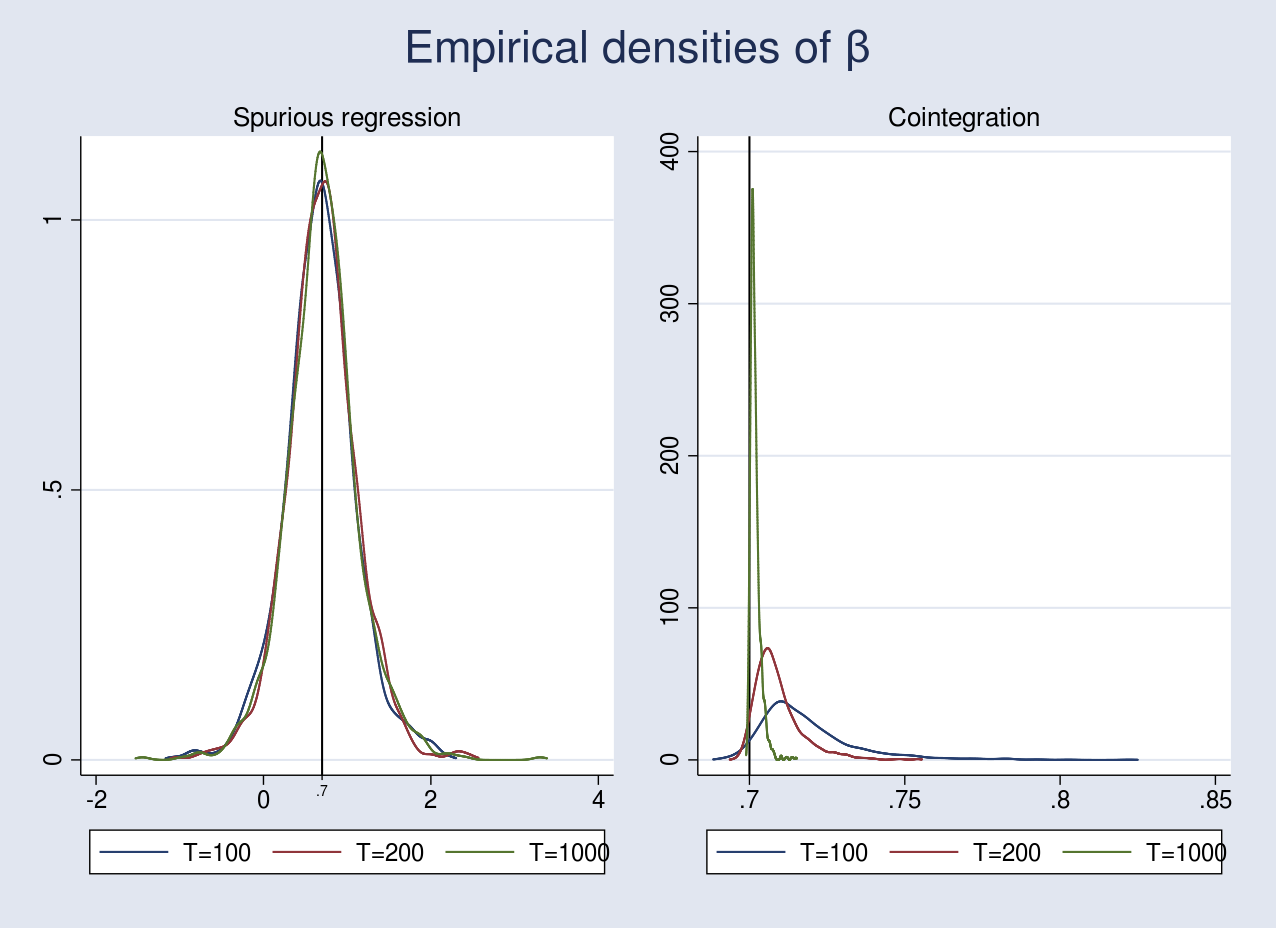
the place (nu_{yt}) and (nu_{xt}) are drawn from a standard distribution with imply 0 and variance matrix ({bf Sigma} = left[begin{matrix} 1 & 0.7 0.7 & 1.5 end{matrix}right]). The graph beneath plots the empirical densities. The code for performing the simulations is supplied within the Appendix.
Within the case of spurious regression, the OLS estimator is inconsistent as a result of it doesn’t converge to its true worth even after rising the pattern measurement from 100 to 1,000. The vertical line at 0.7 represents the true worth of (beta). Furthermore, in finite samples, the coefficients in a spurious regression are often important with a excessive (R^2). In truth, Phillips (1986) confirmed that the (t) and (F) statistics diverge in distribution as (Tto infty), thus making any inferences invalid.
Within the case of cointegration, I artificially launched serial correlation within the error phrases within the data-generating course of. This led to a biased estimate as seen within the graph above for a pattern measurement of 100, which improves barely because the pattern measurement will increase to 200. Remarkably, the OLS estimator converges to its true worth as we enhance the pattern measurement to 1,000. Whereas consistency is a crucial property, we nonetheless can not carry out inference on (hat{beta}) due to its nonstandard asymptotic distribution.
Testing for cointegration
We noticed within the earlier part that the OLS estimator is constant if the collection are cointegrated. That is true even after we fail to account for serial correlation within the error phrases. To check for cointegration, we will assemble residuals primarily based on the static regression and check for the presence of unit root. If the collection are cointegrated, the estimated residuals might be near being stationary. That is the strategy within the Engle–Granger two-step technique. Step one estimates (beta) in eqref{eq1} by OLS adopted by testing for unit root within the residuals. Checks such because the augmented Dickey–Fuller (ADF) or Phillips–Perron (PP) might be carried out on the residuals. Seek advice from an earlier submit for a dialogue of those exams.
The null and various hypotheses for testing cointegration are as follows:
[
H_o: e_t = I(1) qquad H_a: e_t = I(0)
]
The null speculation states that (e_t) is nonstationary, which suggests no cointegration between (y_t) and (x_t). The choice speculation states that (e_t) is stationary and implies cointegration.
If the true cointegrating vector (betab) is understood, then we merely plug its worth in (1) and procure the (e_t) collection. We then apply the ADF check to (e_t). The check statistic could have the usual DF distribution.
Within the case of an unknown cointegrating vector (betab), the ADF check statistic primarily based on the estimated residuals doesn’t observe the usual DF distribution below the null speculation of no cointegration (Phillips and Ouliaris 1990). Moreover, Hansen (1992) reveals that the distribution of the ADF statistic additionally depends upon whether or not (y_t) and (x_t) comprise deterministic phrases reminiscent of constants and time traits. Hamilton (1994, 766) gives vital values for making inference in such instances.
Instance
I’ve two datasets that I saved whereas performing MCS within the earlier part. spurious.dta consists of two variables, (y_t) and (x_t), generated in response to the spurious regression equations in (2). coint.dta additionally consists of (y_t) and (x_t), generated utilizing the cointegration equation in (3).
First, I check for cointegration in spurious.dta.
. use spurious, clear

. reg y x, nocons

      Supply |       SS           df       MS      Variety of obs   =       100
-------------+----------------------------------   F(1, 99)        =      6.20
       Mannequin |  63.4507871         1  63.4507871   Prob > F        =    0.0144
    Residual |  1013.32308        99  10.2355867   R-squared       =    0.0589
-------------+----------------------------------   Adj R-squared   =    0.0494
       Complete |  1076.77387       100  10.7677387   Root MSE        =    3.1993

------------------------------------------------------------------------------
           y |      Coef.   Std. Err.      t    P>|t|     [95% Conf. Interval]
-------------+----------------------------------------------------------------
           x |  -.1257176   .0504933    -2.49   0.014    -.2259073   -.0255279
------------------------------------------------------------------------------
The coefficient on x is adverse and important. I exploit predict with the resid choice to generate the residuals and carry out an ADF check utilizing the dfuller command. I exploit the noconstant choice to supress the fixed time period within the regression and lags(2) to regulate for serial correlation. The noconstant possibility within the dfuller command implies becoming a random stroll mannequin.
. predict spurious_resd, resid

. dfuller spurious_resd, nocons lags(2)

Augmented Dickey-Fuller check for unit root         Variety of obs   =        97

                               ---------- Interpolated Dickey-Fuller ---------
                  Check         1% Crucial       5% Crucial      10% Crucial
               Statistic           Worth             Worth             Worth
------------------------------------------------------------------------------
 Z(t)             -1.599            -2.601            -1.950            -1.610
As talked about earlier, the vital values of the DF distribution is probably not used on this case. The 5% vital worth supplied within the first row of Hamilton (1994, 766) below case 1 in desk B.9 is (-)2.76. The check statistic of (-)1.60 on this case implies failure to reject the null speculation of no cointegration.
I carry out the identical two-step technique for coint.dta beneath.
. use coint, clear

. reg y x, nocons

      Supply |       SS           df       MS      Variety of obs   =       100
-------------+----------------------------------   F(1, 99)        =   3148.28
       Mannequin |  4411.48377         1  4411.48377   Prob > F        =    0.0000
    Residual |   138.72255        99  1.40123788   R-squared       =    0.9695
-------------+----------------------------------   Adj R-squared   =    0.9692
       Complete |  4550.20632       100  45.5020632   Root MSE        =    1.1837

------------------------------------------------------------------------------
           y |      Coef.   Std. Err.      t    P>|t|     [95% Conf. Interval]
-------------+----------------------------------------------------------------
           x |   .7335899   .0130743    56.11   0.000     .7076477    .7595321
------------------------------------------------------------------------------

. predict coint_resd, resid

. dfuller coint_resd, nocons lags(2)

Augmented Dickey-Fuller check for unit root         Variety of obs   =        97

                               ---------- Interpolated Dickey-Fuller ---------
                  Check         1% Crucial       5% Crucial      10% Crucial
               Statistic           Worth             Worth             Worth
------------------------------------------------------------------------------
 Z(t)             -5.955            -2.601            -1.950            -1.610
Evaluating the DF check statistic of (-)5.95 with the suitable vital worth of (-)2.76, I reject the null speculation of no cointegration on the 5% stage.
Conclusion
On this submit, I carried out MCS to point out the consistency of the OLS estimator below cointegration. I used the Engle–Granger two-step strategy to check for cointegration in simulated information.
References
Engle, R. F., and C. W. J. Granger. 1987. Co-integration and error correction: Illustration, estimation, and testing. Econometrica 55: 251–276.
Hamilton, J. D. 1994. Time Collection Evaluation. Princeton: Princeton College Press.
Hansen, B. E. 1992. Effcient estimation and testing of cointegrating vectors within the presence of deterministic traits. Journal of Econometrics 53: 87–121.
Phillips, P. C. B. 1986. Understanding spurious regressions in econometrics. Journal of Econometrics 33: 311–340.
Phillips, P. C. B., and S. Ouliaris. 1990. Asymptotic properties of residual primarily based exams for cointegration. Econometrica 58: 165–193.
Appendix
Code for spurious regression
The next code performs an MCS for a pattern measurement of 100.
cscript
set seed 2016

native MC = 1000

quietly postfile spurious beta_t100 utilizing t100, change

forvalues i=1/`MC' {
        quietly {
                drop _all

                set obs 100
                gen time = _n
                tsset time

                gen nu_y = rnormal(0,0.7)
                gen nu_x = rnormal(0,1.5)

                gen err_y = nu_y in 1
                gen err_x = nu_x in 1
                change err_y = l.err_y + nu_y in 2/l
                change err_x = l.err_x + nu_x in 2/l

                gen y = err_y in 1
                gen x = err_x
                change y = 0.7*x + err_y in 2/l
                if (`i'==1) save spurious, change
                qui reg y x, nocons
        }
                submit spurious (_b[x])
}
postclose spurious
Code for cointegration
The next code performs an MCS for a pattern measurement of 100.
cscript
set seed 2016
native MC = 1000
quietly postfile coint beta_t100 utilizing t100, change
forvalues i=1/`MC' {
quietly {
drop _all
set obs 100
gen time = _n
tsset time
matrix V = (1,0.7�.7,1.5)
drawnorm nu_y nu_x, cov(V)
gen err_y = nu_y in 1
gen err_x = nu_x in 1
change err_y = 0.3*l.nu_y + 0.4*l.nu_x ///
+ nu_y in 2/l
change err_x = 0.7*l.nu_y + 0.1*l.nu_x ///
+ nu_x in 2/l
gen x = err_x in 1
change x = l.x + err_x in 2/l
gen y = 0.7*x + err_y
if (`i'==1) save coint, change
qui reg y x, nocons
}
submit coint (_b[x])
}
postclose coint
Combining graphs
Assuming you’ve gotten run an MCS for pattern sizes of 200 and 1,000, chances are you’ll mix the graph utilizing the next code block.
/*Spurious regression*/
use t100, clear
quietly merge 1:1 _n utilizing t200
drop _merge
quietly merge 1:1 _n utilizing t1000
drop _merge
kdensity beta_t100, n(1000) generate(x_100 f_100) ///
        kernel(gaussian) nograph
label variable f_100 "T=100"
kdensity beta_t200, n(1000) generate(x_200 f_200) ///
        kernel(gaussian) nograph
label variable f_200 "T=200"
kdensity beta_t1000, n(1000) generate(x_1000 f_1000) ///
        kernel(gaussian) nograph
label variable f_1000 "T=1000"
graph twoway (line f_100 x_100) (line f_200 x_200) ///
        (line f_1000 x_1000), legend(rows(1))      ///
        subtitle("Spurious regression")            ///
        saving(spurious, change) xmlabel(0.7)     ///
        xline(0.7, lcolor(black)) nodraw

/*Cointegration*/
use t100, clear
quietly merge 1:1 _n utilizing t200
drop _merge
quietly merge 1:1 _n utilizing t1000
drop _merge
kdensity beta_t100, n(1000) generate(x_100 f_100) ///
        kernel(gaussian) nograph
label variable f_100 "T=100"
kdensity beta_t200, n(1000) generate(x_200 f_200) ///
        kernel(gaussian) nograph
label variable f_200 "T=200"
kdensity beta_t1000, n(1000) generate(x_1000 f_1000) ///
        kernel(gaussian) nograph
label variable f_1000 "T=1000"
graph twoway (line f_100 x_100) (line f_200 x_200) ///
        (line f_1000 x_1000), legend(rows(1))      ///
        subtitle("Cointegration")                  ///
        saving(cointegration, change)             ///
        xline(0.7, lcolor(black)) nodraw

graph mix spurious.gph cointegration.gph,      ///
      title("Empirical densities of {&beta}")