

(defbfy{{bf y}}
defbfA{{bf A}}
defbfB{{bf B}}
defbfu{{bf u}}
defbfI{{bf I}}
defbfe{{bf e}}
defbfC{{bf C}}
defbfsig{{boldsymbol Sigma}})In my final put up, I discusssed estimation of the vector autoregression (VAR) mannequin,
start{align}
bfy_t &= bfA_1 bfy_{t-1} + dots + bfA_k bfy_{t-k} + bfe_t tag{1}
label{var1}
E(bfe_t bfe_t’) &= bfsig label{var2}tag{2}
finish{align}
the place (bfy_t) is a vector of (n) endogenous variables, (bfA_i) are coefficient matrices, (bfe_t) are error phrases, and (bfsig) is the covariance matrix of the errors.
In discussing impulse–response evaluation final time, I briefly mentioned the idea of orthogonalizing the shocks in a VAR—that’s, decomposing the reduced-form errors within the VAR into mutually uncorrelated shocks. On this put up, I’ll go into extra element on orthogonalization: what it’s, why economists do it, and what types of questions we hope to reply with it.
Structural VAR
The straightforward VAR mannequin in eqref{var1} and eqref{var2} supplies a compact abstract of the second-order moments of the information. If all we care about is characterizing the correlations within the knowledge, then the VAR is all we want.
Nevertheless, the reduced-form VAR could also be unsatisfactory for 2 causes, one relating to every equation within the VAR. First, eqref{var1} permits for arbitrary lags however doesn’t enable for contemporaneous relationships amongst its variables. Financial idea typically hyperlinks variables contemporaneously, and if we want to use the VAR to check these theories, it have to be modified to permit for contemporanous relationships among the many mannequin variables. A VAR that does enable for contemporanous relationships amongst its variables could also be written as
start{align}
bfA bfy_t &= bfC_1 bfy_{t-1} + dots + bfC_k bfy_{t-k} + bfe_t
label{var3}tag{3}
finish{align}
and I must introduce new notation (the (bfC_i)) as a result of when (bfA neq bfI), the (bfC_i) will typically differ from the (bfA_i) within the reduced-form VAR. The (bfA) matrix characterizes the contemporaneous relationships among the many variables within the VAR.
The second deficiency of the reduced-form VAR is that its error phrases will, typically, be correlated. We want to decompose these error phrases into mutually orthogonal shocks. Why is orthogonality so vital? After we carry out impulse–response evaluation, we ask the query, “What’s the impact of a shock to at least one equation, holding all different shocks fixed?” To investigate that impulse, we have to hold different shocks fastened. But when the error phrases are correlated, then a shock to at least one equation is related to shocks to different equations; the thought experiment of holding all different shocks fixed can’t be carried out. The answer is to jot down the errors as a linear mixture of “structural” shocks
start{align}
bfe_t &= bfB bfu_t label{var4}tag{4}
finish{align}
With out lack of generality, we will impose (E(bfu_tbfu_t’)=bfI).
So our process, then, is to estimate the parameters of a VAR that has been prolonged to incorporate correlation among the many endogenous variables and exclude correlation among the many error phrases. Mix eqref{var3} and eqref{var4} to acquire the structural VAR mannequin,
start{align}
bfA bfy_t &= bfC_1 bfy_{t-1} + dots + bfC_k bfy_{t-k}
+ bfB bfu_t tag{5}
finish{align}
so the objective is to estimate (bfA), (bfB), and (bfC_i). Sadly, there’s little extra we will say at this stage, as a result of at this stage of generality, the mannequin’s parameters are usually not recognized.
Identification
When the options to population-level second equations are distinctive and produce the true parameters, the parameters are recognized. Within the VAR mannequin, the population-level second situations use the second moments of the variables—variances, covariances, and autocovariances—in addition to the covariance matrix of the error phrases. The identification downside is to maneuver from these moments again to distinctive estimates of the parameters within the structural matrices.
We are able to all the time estimate the reduced-form matrices (bfA_i) and (bfsig) from the VAR in eqref{var1} and eqref{var2}. We are able to then use the knowledge in ((bfA_i,bfsig)) to make inferences about ((bfA,bfB,bfC_i)). What does the structural VAR suggest concerning the reduced-form moments? Assuming that (bfA) is invertible, we will write the structural VAR as
start{align*}
bfy_t &= bfA^{-1} bfC_1 bfy_{t-1}
+ dots
+ bfA^{-1} bfC_k bfy_{t-k}
+ bfA^{-1} bfB bfu_t
finish{align*}
which suggests the next set of relationships,
start{align*}
bfA^{-1}bfC_i &= bfA_i
finish{align*}
for (i=1,2,dots ok), and
start{align*}
bfA^{-1} bfB bfB’ {bfA^{-1}}’ &= bfsig
finish{align*}
If we might kind estimates of (bfA) and (bfB), then recovering the (bfC_i) can be simple.
The issue is that there are lots of (bfA) and (bfB) matrices which might be per the identical noticed (bfsig) matrix. Therefore, with out additional data, we can not uniquely pin down (bfA) and (bfB) from (bfsig).
As a covariance matrix, (bfsig) have to be symmetric and therefore has solely (n(n+1)/2) items of data; nonetheless, (bfA) and (bfB) every have (n^2) parameters. We should place (n^2+n(n-1)/2) restrictions on (bfA) and (bfB) to acquire a singular estimate of (bfA) and (bfB) from (bfsig). The order situation solely ensures that we’ve sufficient restrictions. The rank situation ensures that we’ve sufficient linearly unbiased restrictions. It’s most typical to limit some entries of (bfA) or (bfB) to zero or one.
Cholesky identification
The most typical methodology of identification is to set (bfA=bfI) and to require (bfB) to be a lower-triangular matrix, putting zeros on all entries above the diagonal. This identification scheme locations (n^2) restrictions on (bfA) and locations (n(n-1)/2) restrictions on (bfB), satisfying the order situation. The ensuing mapping from construction to diminished kind is
start{align}
bfB bfB’ = bfsig label{chol}
tag{6}
finish{align}
together with the requirement that (bfB) be decrease triangular. There’s a distinctive lower-triangular matrix (bfB) that satisfies eqref{chol}; therefore, we will uniquely get better the construction from the diminished kind. This identification scheme is usually known as “Cholesky” identification as a result of the matrix (bfB) will be recovered by taking a Cholesky decomposition of (bfsig).
An equal methodology of identification is to let (bfA) be decrease triangular and let (bfB=bfI). Each of those strategies could also be considered imposing a causal ordering on the variables within the VAR: shocks to at least one equation contemporaneously have an effect on variables under that equation however solely have an effect on variables above that equation with a lag. With this interpretation in thoughts, the causal ordering a researcher chooses displays his or her beliefs concerning the relationships amongst variables within the VAR.
Suppose we’ve a VAR with three variables: inflation, the unemployment charge, and the rate of interest. With the ordering (inflation, unemployment, rate of interest), the shock to the inflation equation can have an effect on all variables contemporaneously, however the shock to unemployment doesn’t have an effect on inflation contemporaneously, and the shock to the rate of interest impacts neither inflation nor unemployment contemporaneously. This ordering could mirror some beliefs the researcher has concerning the varied shocks. For instance, if one believes that financial coverage solely impacts different variables with a lag, it’s acceptable to put financial devices just like the rate of interest final within the ordering. Totally different orderings mirror completely different assumptions concerning the underlying construction that the researcher is modeling.
With Cholesky identification, order issues: permuting the variables within the VAR will permute the entries in (bfsig), which in flip will generate completely different (bfB) matrices. The impulse responses one attracts from the mannequin are conditional on the ordering of the variables. One is perhaps tempted, as a type of robustness verify, to attempt a number of orderings to see whether or not impulse responses assorted a lot when the ordering modified. Nevertheless, completely different orderings embed completely different assumptions concerning the relationships amongst variables, and it might or will not be smart to assume that an impulse response might be strong to these differing assumptions.
Instance
Stata’s svar command estimates structural VARs. Let’s revisit the three-variable VAR from the earlier put up, this time utilizing svar. The dataset will be accessed right here. The next code block masses the information, units up the (bfA) and (bfB) matrices, estimates the mannequin, then creates impulse responses and shops them to a file.
. use usmacro.dta
. matrix A1 = (1,0,0 .,1,0 .,.,1)
. matrix B1 = (.,0,0 0,.,0 0,0,.)
. svar inflation unrate ffr, lags(1/6) aeq(A1) beq(B1)
Estimating short-run parameters
Iteration 0: log chance = -708.74354
Iteration 1: log chance = -443.10177
Iteration 2: log chance = -354.17943
Iteration 3: log chance = -303.90081
Iteration 4: log chance = -299.0338
Iteration 5: log chance = -298.87521
Iteration 6: log chance = -298.87514
Iteration 7: log chance = -298.87514
Structural vector autoregression
( 1) [a_1_1]_cons = 1
( 2) [a_1_2]_cons = 0
( 3) [a_1_3]_cons = 0
( 4) [a_2_2]_cons = 1
( 5) [a_2_3]_cons = 0
( 6) [a_3_3]_cons = 1
( 7) [b_1_2]_cons = 0
( 8) [b_1_3]_cons = 0
( 9) [b_2_1]_cons = 0
(10) [b_2_3]_cons = 0
(11) [b_3_1]_cons = 0
(12) [b_3_2]_cons = 0
Pattern: 39 - 236 Variety of obs = 198
Precisely recognized mannequin Log chance = -298.8751
------------------------------------------------------------------------------
| Coef. Std. Err. z P>|z| [95% Conf. Interval]
-------------+----------------------------------------------------------------
/a_1_1 | 1 (constrained)
/a_2_1 | .0348406 .0416245 0.84 0.403 -.046742 .1164232
/a_3_1 | -.3777114 .113989 -3.31 0.001 -.6011257 -.1542971
/a_1_2 | 0 (constrained)
/a_2_2 | 1 (constrained)
/a_3_2 | 1.402087 .1942736 7.22 0.000 1.021318 1.782857
/a_1_3 | 0 (constrained)
/a_2_3 | 0 (constrained)
/a_3_3 | 1 (constrained)
-------------+----------------------------------------------------------------
/b_1_1 | .4088627 .0205461 19.90 0.000 .3685931 .4491324
/b_2_1 | 0 (constrained)
/b_3_1 | 0 (constrained)
/b_1_2 | 0 (constrained)
/b_2_2 | .2394747 .0120341 19.90 0.000 .2158884 .263061
/b_3_2 | 0 (constrained)
/b_1_3 | 0 (constrained)
/b_2_3 | 0 (constrained)
/b_3_3 | .6546452 .0328972 19.90 0.000 .5901679 .7191224
------------------------------------------------------------------------------
. matlist e(A)
| inflation unrate ffr
-------------+---------------------------------
inflation | 1 0 0
unrate | .0348406 1 0
ffr | -.3777114 1.402087 1
. matlist e(B)
| inflation unrate ffr
-------------+---------------------------------
inflation | .4088627
unrate | 0 .2394747
ffr | 0 0 .6546452
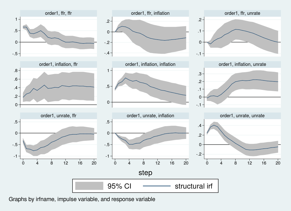
. irf create order1, set(var2.irf) exchange step(20)
(file var2.irf created)
(file var2.irf now lively)
irfname order1 not present in var2.irf
(file var2.irf up to date)
. irf graph sirf, xlabel(0(4)20) irf(order1) yline(0,lcolor(black))
> byopts(yrescale)
The primary two traces arrange the (bfA) and (bfB) matrices. Lacking values in these matrices point out entries to be estimated; entries with given values are assumed to be fastened. I’ve restricted the diagonals of the (bfA) matrix to unity, set components above the primary diagonal to zero, and permit the weather under the primary diagonal to be estimated. In the meantime, I enable the weather on the primary diagonal of the (bfB) matrix to be estimated however limit the remaining entries to zero.
The third line runs the SVAR. The core of svar‘s syntax is acquainted: we specify an inventory of variables and the lag size. The (bfA) and (bfB) matrices are handed to svar by the choices aeq() and beq().
The output of svar focuses on the estimation of the (bfA) and (bfB) matrices; the estimated matrices on lagged endogenous variables are supressed by default. We are able to see that 5 of the six unrestricted entries are statistically important; solely the coefficient on inflation within the unemployment equation (/a_2_1) is statistically insignificant.
The matrices (bfA) and (bfB) could also be of curiosity and will be accessed after estimation in e(A) and e(B). I show these matrices with matlist. You will get a way for a way the impulse responses will behave on impression by inspecting the (bfA) matrix. By building, inflation won’t transfer on impression in response to the opposite two shocks. The unemployment charge will decline barely on impression after an inflation shock, however we’ve already seen within the estimation output that this decline might be statistically insignificant. In the meantime, the rate of interest will rise in response to an increase in inflation however decline in response to an increase within the unemployment charge.
Lastly, I create an irf file, var2.irf, and place the impulse responses into that file below the title order1.
Now, let’s estimate the structural VAR once more however use a special ordering. We are going to place the rate of interest first, then unemployment, then inflation. One strategy to accomplish that’s to set the (bfA) matrix to be higher triangular as a substitute of decrease triangular.
. matrix A2 = (1,.,.  0,1,.  0,0,1)

. matrix B2 = (.,0,0  0,.,0  0,0,.)

. svar inflation unrate ffr, lags(1/6) aeq(A2) beq(B2)
Estimating short-run parameters

Iteration 0:   log chance = -774.35412
Iteration 1:   log chance = -528.28591
Iteration 2:   log chance = -451.41967
Iteration 3:   log chance =  -358.6247
Iteration 4:   log chance = -302.25179
Iteration 5:   log chance = -298.92706
Iteration 6:   log chance = -298.87515
Iteration 7:   log chance = -298.87514

Structural vector autoregression

 ( 1)  [a_1_1]_cons = 1
 ( 2)  [a_2_1]_cons = 0
 ( 3)  [a_2_2]_cons = 1
 ( 4)  [a_3_1]_cons = 0
 ( 5)  [a_3_2]_cons = 0
 ( 6)  [a_3_3]_cons = 1
 ( 7)  [b_1_2]_cons = 0
 ( 8)  [b_1_3]_cons = 0
 ( 9)  [b_2_1]_cons = 0
 (10)  [b_2_3]_cons = 0
 (11)  [b_3_1]_cons = 0
 (12)  [b_3_2]_cons = 0

Pattern:  39 - 236                               Variety of obs     =        198
Precisely recognized mannequin                        Log chance    =  -298.8751

------------------------------------------------------------------------------
             |      Coef.   Std. Err.      z    P>|z|     [95% Conf. Interval]
-------------+----------------------------------------------------------------
      /a_1_1 |          1  (constrained)
      /a_2_1 |          0  (constrained)
      /a_3_1 |          0  (constrained)
      /a_1_2 |  -.0991471    .132311    -0.75   0.454     -.358472    .1601777
      /a_2_2 |          1  (constrained)
      /a_3_2 |          0  (constrained)
      /a_1_3 |  -.1391009   .0419791    -3.31   0.001    -.2213784   -.0568235
      /a_2_3 |   .1449874   .0200558     7.23   0.000     .1056788     .184296
      /a_3_3 |          1  (constrained)
-------------+----------------------------------------------------------------
      /b_1_1 |   .3972748   .0199638    19.90   0.000     .3581464    .4364031
      /b_2_1 |          0  (constrained)
      /b_3_1 |          0  (constrained)
      /b_1_2 |          0  (constrained)
      /b_2_2 |   .2133842    .010723    19.90   0.000     .1923676    .2344008
      /b_3_2 |          0  (constrained)
      /b_1_3 |          0  (constrained)
      /b_2_3 |          0  (constrained)
      /b_3_3 |   .7561185   .0379964    19.90   0.000     .6816469      .83059
------------------------------------------------------------------------------

. matlist e(A)

             | inflation     unrate        ffr
-------------+---------------------------------
   inflation |         1  -.0991471  -.1391009
      unrate |         0          1   .1449874
         ffr |         0          0          1

. matlist e(B)

             | inflation     unrate        ffr
-------------+---------------------------------
   inflation |  .3972748
      unrate |         0   .2133842
         ffr |         0          0   .7561185

. irf create order2, set(var2.irf) exchange step(20)
(file var2.irf now lively)
irfname order2 not present in var2.irf
(file var2.irf up to date)

. irf graph sirf, xlabel(0(4)20) irf(order2) yline(0,lcolor(black))
> byopts(yrescale)
Once more the primary two traces arrange the structural matrices, the third line estimates the VAR, the 2 matlist instructions show the structural matrices, and I create and retailer the related impulse responses. Be aware that I give the impulse responses a reputation, order2, and retailer them in the identical var2.irf file that holds the order1 impulse responses. Then, within the irf graph command, I take advantage of the irf() choice to specify which set of impulse responses I want to graph. On this method, you may retailer a number of impulse responses to the identical file.
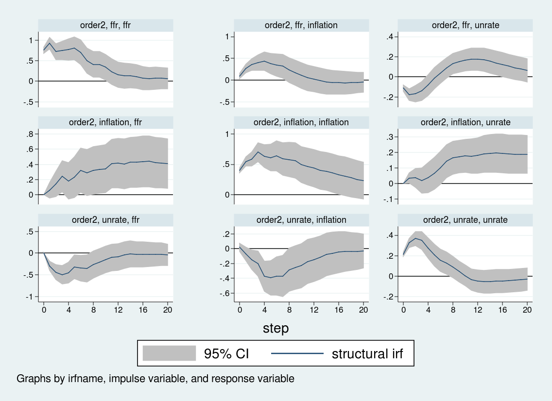
Though among the impulse responses are related, the response of inflation and unemployment to an rate of interest shock differs sharply throughout the 2 orderings. When rates of interest are ordered final, the inflation charge doesn’t reply strongly to rate of interest shocks, whereas the unemployment charge rises over about eight quarters earlier than falling. Against this, when the rate of interest is ordered first, inflation truly rises on an rate of interest shock, and the unemployment charge falls on impression earlier than rising. The impulse response to an rate of interest shock relies upon crucially on the Cholesky ordering.
Conclusion
On this put up, I used svar to estimate a structural VAR and mentioned among the points concerned in estimating the parameters of structural VARs and deciphering their output. Utilizing U.S. macroeconomic knowledge, I confirmed one instance the place completely different identification assumptions produce markedly completely different inferences concerning the conduct of inflation and unemployment to an rate of interest shock.