

In Stata 14.2, we added the flexibility to make use of margins to estimate covariate results after gmm. On this put up, I illustrate find out how to use margins and marginsplot after gmm to estimate covariate results for a probit mannequin.
Margins are statistics calculated from predictions of a beforehand match mannequin at fastened values of some covariates and averaging or in any other case integrating over the remaining covariates. They can be utilized to estimate inhabitants common parameters just like the marginal imply, common remedy impact, or the common impact of a covariate on the conditional imply. I’ll show how utilizing margins is helpful after estimating a mannequin with the generalized methodology of moments.
Probit mannequin
For binary end result (y_i) and regressors ({bf x}_i), the probit mannequin assumes
start{equation}
y_i = {bf 1}({bf x}_i{boldsymbol beta} + epsilon_i > 0) nonumber
finish{equation}
the place the error (epsilon_i) is commonplace regular. The indicator operate ({bf 1}(cdot)) outputs 1 when its enter is true and outputs 0 in any other case.
The conditional imply of (y_i) is
start{equation}
E(y_ivert{bf x}_i) = Phi({bf x}_i{boldsymbol beta}) nonumber
finish{equation}
We are able to use the generalized methodology of moments (GMM) to estimate ({boldsymbol beta}), with pattern second situations
start{equation}
sum_{i=1}^N left[left{ y_i frac{phileft({bf x}_i{boldsymbol beta}right)}{Phileft({bf x}_i{boldsymbol beta}right)} – (1-y_i)
frac{phileft({bf x}_i{boldsymbol beta}right)}{Phileft(-{bf x}_i{boldsymbol beta}right)}right} {bf x}_iright] ={bf 0} nonumber
finish{equation}
Along with the mannequin parameters ({boldsymbol beta}), we may additionally have an interest within the change in (y_i) as we alter one of many covariates in ({bf x}_i). How do people that solely differ within the worth of one of many regressors evaluate?
Suppose we wish to evaluate variations within the regressor (x_{ij}). The vector ({bf x}_{i}^{star}) is ({bf x}_{i}) with the (j)th regressor (x_{ij}) changed by (x_{ij}+1).
The impact of a unit change in (x_{ij}) on (y_i) at ({bf x}_i) is
start{eqnarray*}
E(y_ivert {bf x}_i^{star}) – E(y_ivert {bf x}_i) = Phileft({bf x}_i^{star}{boldsymbol beta}proper) – Phileft({bf x}_i{boldsymbol beta}proper)
finish{eqnarray*}
If we wished to estimate how this impact modified over the inhabitants, we may add the next pattern second situation to our GMM estimation
start{equation}
sum_{i=1}^N delta – left[ Phileft({bf x}_i^{star}{boldsymbol beta}right) – Phileft({bf x}_i{boldsymbol beta}right)right] ={bf 0} nonumber
finish{equation}
This situation implies
start{equation}
delta = frac{1}{N}sum_{i=1}^N Phileft({bf x}_i^{star}{boldsymbol beta}proper) – Phileft({bf x}_i{boldsymbol beta}proper) ={bf 0} nonumber
finish{equation}
Reasonably than utilizing the situation for (delta) within the GMM estimation, we are able to straight calculate the pattern common of the impact after estimation.
start{equation}
hat{delta} = frac{1}{N} sum_{i=1}^N Phileft({bf x}_i^{star}widehat{boldsymbol beta}proper) – Phileft({bf x}_iwidehat{boldsymbol beta}proper) nonumber
finish{equation}
The usual error for this imply impact must be adjusted for the estimation of ({boldsymbol beta}). We are able to use gmm to estimate ({boldsymbol beta}) after which use margins to estimate (delta) and its correctly adjusted commonplace error. This supplies flexibility. You may estimate a mannequin with few second situations after which estimate a number of margins.
Covariate results
We estimate the imply results for a probit regression mannequin utilizing gmm and margins from simulated knowledge. We regress the binary (y_i) on binary (d_i) and steady (x_i) and (z_i). A quadratic time period for (x_i) is included within the mannequin, and we work together each powers of (x_i) and (z_i) with (d_i).
First, we use gmm to estimate ({boldsymbol beta}). Issue-variable notation is used to specify the quadratic energy of (x_i) and the interactions of the powers of (x_i) and (z_i) with (d_i).
. gmm (cond(y,normalden({y: i.d##(c.x c.x#c.x c.z) i.d _cons})/
>         regular({y:}),-normalden({y:})/regular(-{y:}))),
>         devices(i.d##(c.x c.x#c.x c.z) i.d) onestep

Step 1
Iteration 0:   GMM criterion Q(b) =  .26129294
Iteration 1:   GMM criterion Q(b) =  .01621062
Iteration 2:   GMM criterion Q(b) =  .00206357
Iteration 3:   GMM criterion Q(b) =  .00033537
Iteration 4:   GMM criterion Q(b) =  4.916e-06
Iteration 5:   GMM criterion Q(b) =  1.539e-08
Iteration 6:   GMM criterion Q(b) =  3.361e-13

notice: mannequin is strictly recognized

GMM estimation

Variety of parameters =   8
Variety of moments    =   8
Preliminary weight matrix: Unadjusted                 Variety of obs   =      5,000

------------------------------------------------------------------------------
             |               Strong
             |      Coef.   Std. Err.      z    P>|z|     [95% Conf. Interval]
-------------+----------------------------------------------------------------
         1.d |   1.752056   .0987097    17.75   0.000     1.558588    1.945523
           x |   .2209241   .0311227     7.10   0.000     .1599247    .2819235
             |
     c.x#c.x |  -.2864622   .0199842   -14.33   0.000    -.3256305   -.2472939
             |
           z |  -.6813765   .0558371   -12.20   0.000    -.7908152   -.5719379
             |
       d#c.x |
          1  |    .311213   .0543018     5.73   0.000     .2047835    .4176426
             |
   d#c.x#c.x |
          1  |  -.7297855   .0513903   -14.20   0.000    -.8305086   -.6290624
             |
       d#c.z |
          1  |  -.4272026   .0807842    -5.29   0.000    -.5855368   -.2688684
             |
       _cons |   .1180114   .0520303     2.27   0.023     .0160339    .2199888
------------------------------------------------------------------------------
Devices for equation 1: 0b.d 1.d x c.x#c.x z 0b.d#co.x 1.d#c.x 0b.d#co.x#co.x 1.d#c.x#c.x 0b.d#co.z
    1.d#c.z _cons
Now, we use margins to estimate the imply impact of fixing (x_i) to (x_i+1). We specify vce(unconditional) to estimate the imply impact over the inhabitants of (x_i), (z_i), and (d_i). The conventional chance expression is specified within the expression() choice. The expression operate xb() is used to get the linear prediction. We specify the at(generate()) choice and atcontrast(r) beneath the distinction choice in order that the expression at (x_i) might be subtracted from the expression at (x_i+1). nowald is specified to suppress the Wald check of the distinction.
. margins, at(x=generate(x)) at(x=generate(x+1)) vce(unconditional)
>         expression(regular(xb())) distinction(atcontrast(r) nowald)

Contrasts of predictive margins

Expression   : regular(xb())

1._at        : x               = x

2._at        : x               = x+1

--------------------------------------------------------------
             |            Unconditional
             |   Distinction   Std. Err.     [95% Conf. Interval]
-------------+------------------------------------------------
         _at |
   (2 vs 1)  |  -.0108121   .0040241     -.0186993    -.002925
--------------------------------------------------------------
Unit adjustments are notably helpful for evaluating the impact of discrete covariates. When a discrete covariate is specified utilizing factor-variable notation, we are able to use distinction notation in margins to estimate the covariate impact.
We estimate the imply impact of fixing from (d_i=0) to (d_i=1) over the inhabitants of covariates with margins. We specify the distinction r.d and the conditional imply within the expression() choice. The expression might be evaluated at (d_i=0) after which subtracted from the expression evaluated at (d_i=1). We specify distinction(nowald) to suppress the Wald check of the distinction.
. margins r.d, expression(regular(xb())) vce(unconditional) distinction(nowald)

Contrasts of predictive margins

Expression   : regular(xb())

--------------------------------------------------------------
             |            Unconditional
             |   Distinction   Std. Err.     [95% Conf. Interval]
-------------+------------------------------------------------
           d |
   (1 vs 0)  |   .1370625   .0093206      .1187945    .1553305
--------------------------------------------------------------
So on common over the inhabitants, altering from (d_i=0) to (d_i=1) and protecting different covariates fixed will improve the chance of success by 0.14.
Graphing covariate results
Now we have used margins to estimate the imply covariate impact over the inhabitants of covariates. We are able to additionally use margins to estimate covariate results at fastened values of the opposite covariates or to common the covariate impact over sure covariates whereas fixing others. We might study a number of results to discover a sample. The marginsplot command graphs results estimated by margins and may be useful in these conditions.
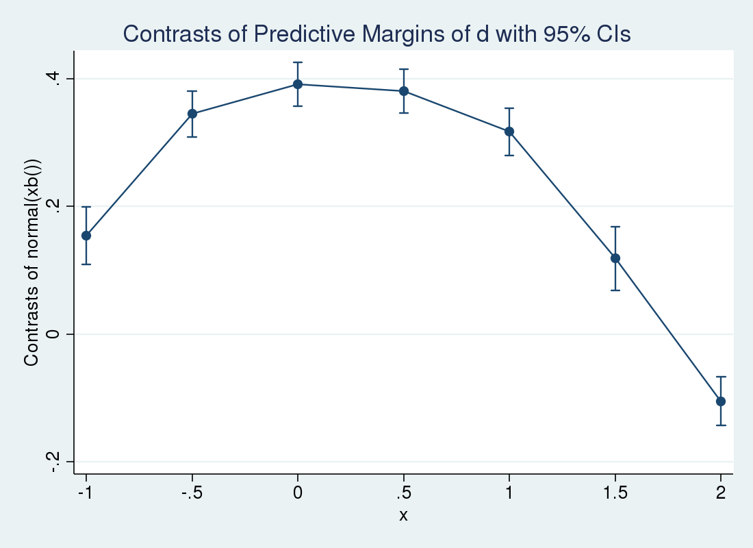
Suppose we wished to see how the impact of a unit change in (d_i) various over (x_i). We are able to use margins with the at() choice to estimate the impact at completely different values of (x_i), averaged over the opposite covariates. We suppress the legend of fastened covariate values by specifying noatlegend.
. margins r.d, at(x = (-1 -.5 0 .5 1 1.5 2))
>         expression(regular(xb())) noatlegend
>         vce(unconditional) distinction(nowald)

Contrasts of predictive margins

Expression   : regular(xb())

--------------------------------------------------------------
             |            Unconditional
             |   Distinction   Std. Err.     [95% Conf. Interval]
-------------+------------------------------------------------
       d@_at |
 (1 vs 0) 1  |   .1536608   .0230032      .1085753    .1987462
 (1 vs 0) 2  |   .3446265   .0184594      .3084468    .3808062
 (1 vs 0) 3  |   .3907978    .017575      .3563515    .4252441
 (1 vs 0) 4  |   .3802466    .017735      .3454866    .4150066
 (1 vs 0) 5  |   .3166307   .0189175      .2795531    .3537083
 (1 vs 0) 6  |   .1182164   .0252829      .0686628      .16777
 (1 vs 0) 7  |  -.1053685   .0193225     -.1432399   -.0674971
--------------------------------------------------------------
The marginsplot command will graph these outcomes for us.
. marginsplot

  Variables that uniquely determine margins: x
So the impact will increase over small (x_i) and reduces as (x_i) grows giant. We are able to use margins and marginsplot once more to look at the conditional means at completely different values of (x_i). This time, we specify the over() choice in order that separate predictions are made for (d_i=1) and (d_i=0). We count on to see the strains cross at a sure level, because the covariate impact crossed zero within the earlier plot.
. margins, at(x = (-1 -.5 0 .5 1 1.5 2)) over(d)
>         expression(regular(xb())) noatlegend
>         vce(unconditional)

Predictive margins                              Variety of obs     =      5,000

Expression   : regular(xb())
over         : d

------------------------------------------------------------------------------
             |            Unconditional
             |     Margin   Std. Err.      z    P>|z|     [95% Conf. Interval]
-------------+----------------------------------------------------------------
       _at#d |
        1 0  |   .2117609    .013226    16.01   0.000     .1858384    .2376834
        1 1  |   .3602933   .0194334    18.54   0.000     .3222046    .3983819
        2 0  |   .3042454   .0135516    22.45   0.000     .2776847    .3308061
        2 1  |   .6421908   .0142493    45.07   0.000     .6142627    .6701188
        3 0  |   .3616899   .0145202    24.91   0.000     .3332308     .390149
        3 1  |   .7455187   .0121556    61.33   0.000     .7216941    .7693432
        4 0  |      .3743    .014849    25.21   0.000     .3451965    .4034035
        4 1  |   .7475205   .0120208    62.19   0.000     .7239601    .7710809
        5 0  |   .3406649    .014334    23.77   0.000     .3125709     .368759
        5 1  |   .6504099   .0141534    45.95   0.000     .6226699      .67815
        6 0  |   .2651493   .0141303    18.76   0.000     .2374545    .2928442
        6 1  |   .3777989   .0215394    17.54   0.000     .3355825    .4200153
        7 0  |   .1642177    .014551    11.29   0.000     .1356982    .1927372
        7 1  |   .0565962   .0128524     4.40   0.000      .031406    .0817864
------------------------------------------------------------------------------

. marginsplot

  Variables that uniquely determine margins: x d
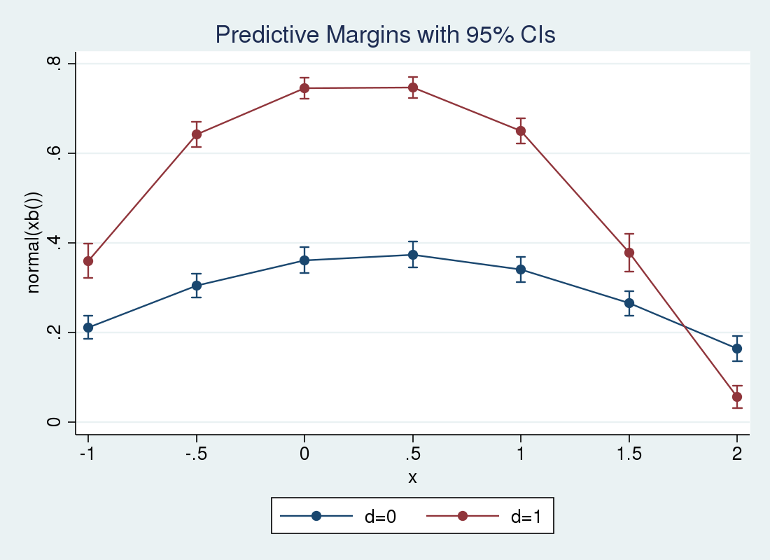
We see that the conditional means for (d_{i}=0) rise above the means for (d_{i}=0) at barely under (x_i = 1.75).
Differential results
As a substitute of a unit change, we could also be within the differential impact. That is the normalized impact on the imply of a small change within the covariate, the spinoff of the imply with regard to the covariate (x_{ij}). That is referred to as the marginal or partial impact of (x_{ij}) on (E(y_ivert {bf x}_i)). See part 2.2.5 of Wooldridge (2010), part 5.2.4 of Cameron and Trivedi (2005), or part 10.6 of Cameron and Trivedi (2010) for extra particulars. We are able to estimate the partial impact utilizing margins, at fastened values of the regressors, or the imply partial impact over the inhabitants or pattern.
We are going to use margins to estimate the imply marginal results for the continual covariates over the inhabitants of covariates. margins will take the derivatives for us if we specify dydx(). We solely have to specify the type of the prediction. We once more use the expression() choice for this objective.
. margins, expression(regular(xb())) vce(unconditional) dydx(x z)

Common marginal results                        Variety of obs     =      5,000

Expression   : regular(xb())
dy/dx w.r.t. : x z

------------------------------------------------------------------------------
             |            Unconditional
             |      dy/dx   Std. Err.      z    P>|z|     [95% Conf. Interval]
-------------+----------------------------------------------------------------
           x |   .0121859   .0045472     2.68   0.007     .0032736    .0210983
           z |  -.1439682   .0062519   -23.03   0.000    -.1562217   -.1317146
------------------------------------------------------------------------------
Conclusion
On this put up, I’ve demonstrated find out how to use margins after gmm to estimate covariate results for probit fashions. I additionally demonstrated how marginsplot can be utilized to graph covariate results.
In future posts, we’ll use margins and marginsplot after gmm freely. This may allow us to carry out marginal estimation and hold our second situations from changing into overcomplicated.
Appendix 1
The next code was used to generate the probit regression knowledge.
. set seed 34

. quietly set obs 5000

. generate double x = 2*rnormal() + .1

. generate byte d = runiform() > .5

. generate double z = rchi2(1)

. generate double y = .2*x +.3*d*x - .3*(x^2) -.7*d*(x^2)
>         -.8*z -.2*z*d + .2 + 1.5*d + rnormal() > 0
References
Cameron, A. C., and P. Okay. Trivedi. 2005. Microeconometrics: Strategies and Purposes. New York: Cambridge College Press.
——. 2010. Microeconometrics Utilizing Stata. Rev. ed. School Station, TX: Stata Press.
Wooldridge, J. M. 2010. Econometric Evaluation of Cross Part and Panel Information. 2nd ed. Cambridge, MA: MIT Press.