KV Cache Optimization by way of Multi-Head Latent Consideration

Desk of Contents

KV Cache Optimization by way of Multi-Head Latent Consideration
Recap of KV Cache
- The Want for KV Cache Optimization
Multi-Head Latent Consideration (MLA)
PyTorch Implementation of Multi-Head Latent Consideration
Abstract
- Quotation Data

KV Cache Optimization by way of Multi-Head Latent Consideration

Transformer-based language fashions have lengthy relied on Key-Worth (KV) caching to speed up autoregressive inference. By storing beforehand computed key and worth tensors, fashions keep away from redundant computation throughout decoding steps. Nonetheless, as sequence lengths develop and mannequin sizes scale, the reminiscence footprint and compute value of KV caches develop into more and more prohibitive — particularly in deployment eventualities that demand low latency and excessive throughput.

Current improvements, corresponding to Multi-head Latent Consideration (MLA), notably explored in DeepSeek-V2, provide a compelling different. As an alternative of caching full-resolution KV tensors for every consideration head, MLA compresses them right into a shared latent house utilizing low-rank projections. This not solely reduces reminiscence utilization but in addition permits extra environment friendly consideration computation with out sacrificing mannequin high quality.

Impressed by this paradigm, this publish dives into the mechanics of KV cache optimization by MLA, unpacking its core parts: low-rank KV projection, up-projection for decoding, and a novel twist on rotary place embeddings (RoPE) that decouples positional encoding from head-specific KV storage.

By the top, you’ll see how these strategies converge to kind a leaner, quicker consideration mechanism — one which preserves expressivity whereas dramatically enhancing inference effectivity.

This lesson is the 2nd of a 3-part collection on LLM Inference Optimization 101 — KV Cache:

Introduction to KV Cache Optimization Utilizing Grouped Question Consideration
KV Cache Optimization by way of Multi-Head Latent Consideration (this tutorial)
KV Cache Optimization by way of Tensor Product Consideration

To learn to optimize KV Cache utilizing Multi-Head Latent Consideration, simply hold studying.

Searching for the supply code to this publish?

Leap Proper To The Downloads Part

Recap of KV Cache

Transformers, particularly in giant language fashions (LLMs), have develop into the dominant paradigm for sequence modeling in language, imaginative and prescient, and multimodal AI. On the coronary heart of scalable inference in such fashions lies the Key-Worth (KV) cache, a mechanism central to environment friendly autoregressive decoding.

As transformers generate textual content (or different sequences) one token at a time, the eye mechanism computes, caches, after which reuses key (Ok) and worth (V) vectors for all beforehand seen tokens within the sequence. This allows the mannequin to keep away from redundant recomputation, lowering each the computational time and power required to generate every new token.

Technically, for an enter sequence of size $L$ , at every layer and for every consideration head, the mannequin produces queries $Q$ , keys $K$ , and values $V$ . In basic Multi-Head Consideration (MHA), the computation for a single consideration head is:

$text{Attention}(Q, K, V) = text{softmax}left(dfrac{Q K^top}{sqrt{d_k}}right) V,$

the place $d_k$ is the dimension of the important thing and question vectors per head. The necessity to attend to all earlier tokens for each new token pushes computational complexity from $O(n^2)$ (with out caching) to $O(n)$ (with caching), the place $n$ is sequence size.

Throughout autoregressive inference, caching is essential. For every new token, the beforehand computed Ok and V vectors from all prior tokens are saved and reused; new Ok/V for the just-generated token are added to the cache. The method will be summarized in a easy workflow:

For the primary token, compute and cache Ok/V
When producing additional tokens:
- Compute Q for the present token
- Retrieve all cached Ok/V
- Compute consideration utilizing present Q and cached Ok/V
- Replace the cache with the brand new Ok/V

Regardless of its easy magnificence in enabling linear-time decoding, the KV cache rapidly turns into a bottleneck in large-scale, long-context fashions. Its reminiscence utilization scales as:

$text{Memory}_{text{KV}} = L times n_{text{heads}} times (d_k + d_v) times text{Layers} times text{Precision}$

This could simply attain dozens of gigabytes for high-end LLMs, typically dwarfing the house wanted only for mannequin weights. For example, in Llama-2-7B with a context window of 28,000 tokens, KV cache use is similar to mannequin weights — about 14 GB in FP16.

A direct result’s that inference efficiency is not bounded solely by compute — it turns into sure by reminiscence bandwidth and capability. On present GPUs, the bottleneck shifts from floating-point ops to studying and writing very broad matrices because the token context expands. Autoregressive era, already a sequential (non-parallel) course of, will get additional constrained.

The Want for KV Cache Optimization

To maintain up with LLMs deployed for real-world dialogue, code assistants, and doc summarization — typically requiring context lengths of 32K tokens and past — an environment friendly KV cache is indispensable. Fashionable software program frameworks corresponding to Hugging Face Transformers, NVIDIA’s FasterTransformer, and vLLM assist numerous cache implementations and quantization methods to optimize this significant element.

Nonetheless, as context home windows improve, merely quantizing or sub-sampling cache entries proves inadequate; the redundancy within the hidden dimension of Ok/V stays untapped, leaving additional optimization potential on the desk.

That is the place Multi-Head Latent Consideration (MLA) steps in — it optimizes KV cache storage and reminiscence bandwidth by way of clever, mathematically sound low-rank and latent house projections, enabling transformers to function effectively in long-context, high-throughput settings.

Multi-Head Latent Consideration (MLA)

Low-Rank KV Projection

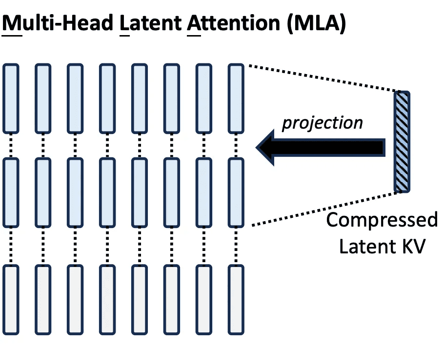
The guts of MLA’s effectivity lies in low-rank projection, a method that reduces the dimensionality of Ok/V tensors earlier than caching. Slightly than storing full-resolution Ok/V vectors for every head and every token, MLA compresses them right into a shared latent house, leveraging the underlying linear redundancy of pure language and the overparameterization of transformer blocks (Determine 1).

Mathematical Foundations

In commonplace MHA, for enter sequence $X in mathbb{R}^{L times D_{text{model}}}$ and $n_h$ heads, Q, Ok, V are projected as:

$Q = X W^Q;quad K = X W^K;quad V = X W^V text{ where } W^Q, W^K, W^V in mathbb{R}^{D_{text{model}} times n_h cdot d_h}$

the place $d_h$ is the pinnacle dimension. Autoregressive inference makes it essential to cache Ok and V for all previous steps, resulting in a big cache matrix of form $(L, n_h, d_h)$ per layer and per sort (Ok/V).

MLA innovates by introducing latent down-projection matrices:

$Q_l = X W^Q_{text{down}}; quad C_{KV,l} = X W^{KV}_{text{down}}$

the place $W^Q_{text{down}} in mathbb{R}^{D_{text{model}} times D_{Q_l}}; quad W^{KV}_{text{down}} in mathbb{R}^{D_{text{model}} times D_{KV_l}}$

Right here, the mannequin tasks Q, Ok, and V into lower-dimensional latent areas, the place $D_{Q_l}, D_{KV_l}$ are considerably smaller than the unique dimensions.

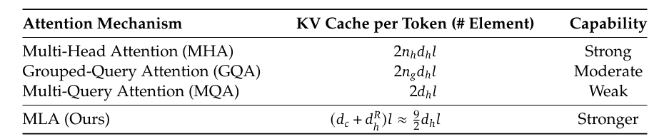
In apply, for a 4096-dimensional mannequin with 32 heads, every with 128 dimensions per head, the usual KV cache requires 4096 values per token per sort. MLA reduces this to (e.g., 512 values per token), delivering an 8x discount in cache dimension (Desk 1).

**Desk 1:** KV Cache dimension per token for various consideration mechanisms (supply: Li, 2025).

Up-Projection

After compressing Ok and V right into a shared, low-dimensional latent house, MLA should reconstruct (“up-project”) the total Ok and V representations when wanted for consideration computations. This on-demand up-projection is what permits the mannequin to reap storage and bandwidth financial savings, but retain excessive representational and modeling capability.

As soon as the sequence has been projected into latent areas ( $C_{KV}$ for Ok and V, $C_Q$ for Q):

$Q = Q_l W^Q_{text{up}};quad K = C_{KV,l} W^K_{text{up}};quad V = C_{KV,l} W^V_{text{up}}$

the place:

$Q_l$ and $C_{KV,l}$ are low-dimensional latent representations,
$W^Q_{text{up}}, W^K_{text{up}}, W^V_{text{up}}$ are decompression matrices.

When computing the eye rating:

$O_i = text{softmax} left( dfrac{Q K^top}{sqrt{d_k}} right)V = text{softmax}left( dfrac{C_Q W^{Q_{text{up}},i} left({W^{K_{text{up}},i}}right)^top}{sqrt{d_k}}right)C_{KV} W^{V_text{up},i}$

the place:

Down-projection: Compresses $X$ to $C_Q$ , $C_text{KV}$ ,
Up-projection: Reprojects the latent house to go dimensions by way of the decompression/up-projection matrices.

Importantly, the multiplication $W^{Q_{text{up}},i} left({W^{K_{text{up}},i}}right)^top$ is impartial of the enter and will be precomputed, additional saving consideration computation at inference.

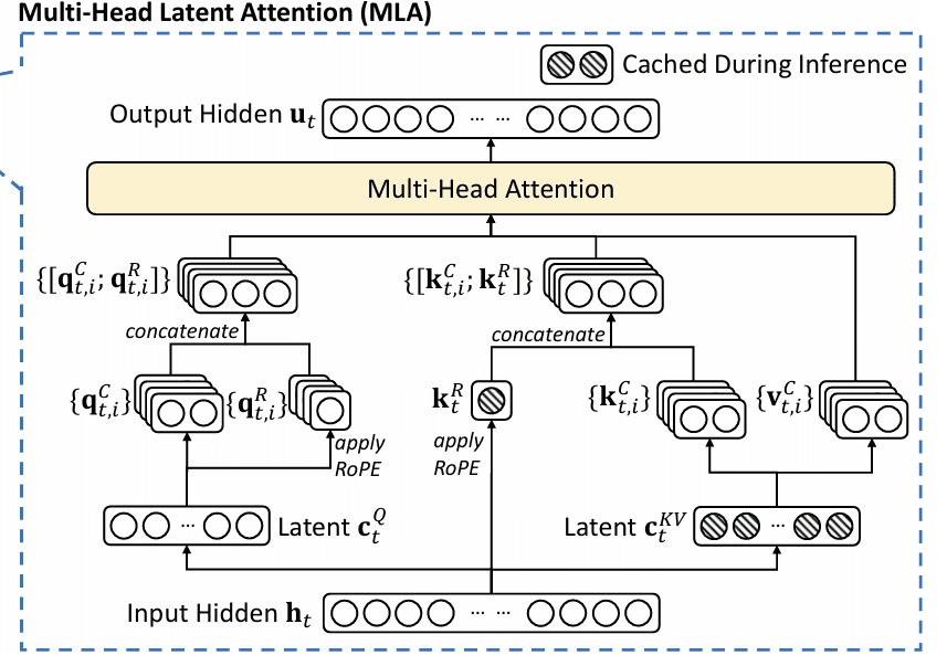
This optimizes each storage (cache solely latent vectors) and compute (precompute and cache up-projection weights) (Determine 2).

**Determine 2:** Multi-Head Latent Consideration (supply: Li, 2025).

Decoupled Rotary Place Embeddings (RoPE)

Place info is the essential ingredient for transformer consideration to respect the order of sequences, whether or not tokens in textual content or patches in pictures. Early transformers used absolute or relative place encodings, however these typically fell quick for long-range or extrapolative contexts.

Rotary Place Embedding (RoPE) is the fashionable resolution, utilized in main LLMs (LLAMA, Qwen, Gemma, and so forth.), leveraging a mathematical trick: place is encoded as a section rotation in every even-odd pair of embedding dimensions, so the dot product between question and key captures relative place because the angular distinction — elegant, parameter-free, and future-proof for lengthy contexts.

RoPE in Normal MHA

Formally, for token place $p$ and embedding index $i$ :

$text{RoPE for dim-pair} left( x^{(2i)}, x^{(2i+1)} right) = left( begin{bmatrix} cos(theta_{p,i}) & -sin(theta_{p,i}) sin(theta_{p,i}) & cos(theta_{p,i}) end{bmatrix} begin{bmatrix} x^{(2i)} x^{(2i+1)} end{bmatrix} right)$ with $( theta_{p,i} )$

decided analytically for every pair and place.

This rotation ensures that the relative place (i.e., the gap between tokens) drives the similarity in consideration, enabling highly effective extrapolation for long-context and relative reasoning.

Challenges in MLA: The Want for Decoupling

In MLA, the problem is that the low-rank compression and up-projection pipeline can not “commute” previous the nonlinear rotational operation inherent to RoPE. That’s, merely projecting Ok/V right into a latent house and reconstructing later is incompatible with making use of the rotation in the usual method post-compression.

To handle this, Decoupled RoPE is launched:

Break up the important thing and question representations into positional and non-positional (NoPE) parts earlier than compression
Apply RoPE solely to the positional parts (sometimes a subset of the pinnacle dimensions)
Depart the majority of the compressed, latent representations unrotated
Concatenate these earlier than last consideration rating computation

Mathematically, for head $s$ :

$k_i^{(s)} = (c_i W_{kc}^{(s)}) oplus (x_i W_{kr} mathcal{R}_i)$

the place $oplus$ is concatenation, $c_i$ is the low-rank latent vector, $W_{kc}^{(s)}$ is head-specific up-projection, $W_{kr}$ is projection to the RoPE subspace, and $mathcal{R}_i$ is the rotation matrix at place $i$ .

Queries are handled analogously. This break up permits MLA’s reminiscence effectivity whereas preserving RoPE’s highly effective relative place encoding.

PyTorch Implementation of Multi-Head Latent Consideration

On this part, we are going to see how utilizing Multi-head Latent Consideration improves the KV Cache dimension. For simplicity, we are going to implement a toy transformer mannequin with 1 layer of RoPE-less Multi-Head Latent Consideration.

Multi-Head Latent Consideration

We’ll begin by implementing the Multi-head Latent Consideration in PyTorch. For simplicity, we are going to use a RoPE-less variant of Multi-head Latent Consideration on this implementation.

import torch
import torch.nn as nn
import time
import matplotlib.pyplot as plt
import math

class MultiHeadLatentAttention(nn.Module):
    def __init__(self, d_model=4096, num_heads=128, q_latent_dim=12, kv_latent_dim=4):
        tremendous().__init__()
        self.d_model = d_model
        self.num_heads = num_heads
        self.q_latent_dim = q_latent_dim
        self.kv_latent_dim = kv_latent_dim
        head_dim = d_model // num_heads

        # Question projections
        self.Wq_d = nn.Linear(d_model, q_latent_dim)

        # Precomputed matrix multiplications of W_q^U and W_k^U, for a number of heads
        self.W_qk = nn.Linear(q_latent_dim, num_heads * kv_latent_dim)

        # Key/Worth latent projections
        self.Wkv_d = nn.Linear(d_model, kv_latent_dim)
        self.Wv_u = nn.Linear(kv_latent_dim, num_heads * head_dim)

        # Output projection
        self.Wo = nn.Linear(num_heads * head_dim, d_model)

    def ahead(self, x, kv_cache):
        batch_size, seq_len, d_model = x.form

        # Projections of enter into latent areas
        C_q = self.Wq_d(x)     # form: (batch_size, seq_len, q_latent_dim)
        C_kv = self.Wkv_d(x)   # form: (batch_size, seq_len, kv_latent_dim)

        # Append to cache
        kv_cache['kv'] = torch.cat([kv_cache['kv'], C_kv], dim=1)

        # Develop KV heads to match question heads
        C_kv = kv_cache['kv']
        # print(C_kv.form)

        # Consideration rating, form: (batch_size, num_heads, seq_len, seq_len)
        C_qW_qk = self.W_qk(C_q).view(batch_size, seq_len, self.num_heads, self.kv_latent_dim)
        scores = torch.matmul(C_qW_qk.transpose(1, 2), C_kv.transpose(-2, -1)[:, None, ...]) / math.sqrt(self.kv_latent_dim)

        # Consideration computation
        attn_weight = torch.softmax(scores, dim=-1)
        # Restore V from latent house
        V = self.Wv_u(C_kv).view(batch_size, C_kv.form[1], self.num_heads, -1)
        # Compute consideration output, form: (batch_size, seq_len, num_heads, head_dim)
        output = torch.matmul(attn_weight, V.transpose(1,2)).transpose(1,2).contiguous()
        # Concatentate the heads, then apply output projection
        output = self.Wo(output.view(batch_size, seq_len, -1))
        return output, kv_cache

This implementation defines a customized PyTorch module for Multi-head Latent Consideration (MLA), a memory-efficient variant of normal multi-head consideration. On Traces 1-5, we import the mandatory libraries, together with PyTorch and matplotlib for potential visualization. The category MultiHeadLatentAttention begins on Line 7, the place we initialize key hyperparameters: the mannequin dimension d_model, variety of heads, and latent dimensions for queries (q_latent_dim) and keys/values (kv_latent_dim).

Notably, d_model is about to 4096, suggesting a high-dimensional enter house. On Traces 17-27, we outline the projection layers: Wq_d maps enter to a low-dimensional question latent house, W_qk transforms queries into head-specific key projections, Wkv_d compresses enter into latent KV representations, and Wv_u restores values from latent house for consideration output. The ultimate layer Wo tasks concatenated consideration outputs again to the mannequin dimension.

Within the ahead technique beginning on Line 29, we course of the enter tensor x and a operating kv_cache. On Traces 30-34, we challenge the enter into question (C_q) and KV (C_kv) latent areas. The KV cache is up to date on Line 37 by appending the brand new latent KV representations. On Traces 44 and 45, we compute consideration scores by projecting queries into head-specific key areas (C_qW_qk) and performing scaled dot-product consideration in opposition to the cached latent keys. This yields a rating tensor of form (batch_size, num_heads, seq_len, seq_len).

On Line 48, we apply softmax to get consideration weights and up-project the cached latent values (C_kv) into full-resolution per-head worth tensors (V). The ultimate output is computed by way of a weighted sum of values, reshaped, and handed by the output projection layer on Traces 50-54.

Toy Transformer and Inference

Now that we’ve got carried out the multi-head latent consideration module, we are going to implement a 1-layer toy Transformer block that takes a sequence of enter tokens, together with KV Cache, and performs a single feedforward cross.

class TransformerBlock(nn.Module):
    def __init__(self,  d_model=128*128, num_heads=128, q_latent_dim=12, kv_latent_dim=4):
        tremendous().__init__()
        self.attn = MultiHeadLatentAttention(d_model, num_heads, q_latent_dim, kv_latent_dim)
        self.norm1 = nn.LayerNorm(d_model)
        self.ff = nn.Sequential(
            nn.Linear(d_model, d_model * 4),
            nn.ReLU(),
            nn.Linear(d_model * 4, d_model)
        )
        self.norm2 = nn.LayerNorm(d_model)

    def ahead(self, x, kv_cache):
        attn_out, kv_cache = self.attn(x, kv_cache)
        x = self.norm1(x + attn_out)
        ff_out = self.ff(x)
        x = self.norm2(x + ff_out)
        return x, kv_cache

We outline a TransformerBlock class on Traces 1-11, the place the constructor wires collectively a MultiHead Latent Consideration layer (self.attn), two LayerNorms (self.norm1 and self.norm2), and a two-layer feed-forward community (self.ff) that expands the hidden dimension by 4× after which tasks it again.

On Traces 13-18, the ahead technique takes enter x and the kv_cache, runs x by the eye module to get attn_out and an up to date cache, then applies a residual connection plus layer norm (x = norm1(x + attn_out)). Subsequent, we feed this by the FFN, add one other residual connection, normalize once more (x = norm2(x + ff_out)), and at last return the reworked hidden states alongside the refreshed kv_cache.

Subsequent, the code snippet under runs an inference to generate a sequence of tokens in an autoregressive method.

def run_inference(block):
    d_model = block.attn.d_model
    num_heads = block.attn.num_heads
    kv_latent_dim = block.attn.kv_latent_dim

    seq_lengths = checklist(vary(1, 101, 10))
    kv_cache_sizes = []
    inference_times = []

    kv_cache = {
        'kv': torch.empty(1, 0, kv_latent_dim)
    }

    for seq_len in seq_lengths:
        x = torch.randn(1, 1, d_model)  # One token at a time
        begin = time.time()
        o, kv_cache = block(x, kv_cache)
        finish = time.time()
        # print(o.form)
        dimension = kv_cache['kv'].numel()
        kv_cache_sizes.append(dimension)
        inference_times.append(finish - begin)

    return seq_lengths, kv_cache_sizes, inference_times

On Traces 1-8, we outline run_inference, pull out d_model, num_heads, and kv_latent_dim, and construct a listing of goal seq_lengths (1 to 101 in steps of 10), together with empty lists for kv_cache_sizes and inference_times. On Traces 10-12, we initialize kv_cache with empty tensors for 'kv' of form [1, 0, kv_latent_dim] so it may develop as we generate tokens.

Then, within the loop over every seq_len on Traces 14-18, we simulate feeding one random token x at a time into the transformer block, timing the ahead cross, and updating kv_cache. Lastly, on Traces 20-24, we measure the full variety of components within the cached keys and values, append that to kv_cache_sizes, report the elapsed time to inference_times, and on the finish return all three lists for plotting or evaluation.

Experiments and Evaluation

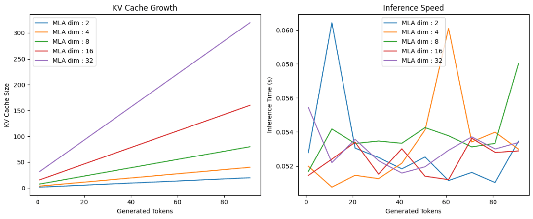
Lastly, we are going to take a look at our implementation of multi-head latent consideration with totally different KV latent dimensions. For every latent dimension, we are going to plot the dimensions of the KV Cache and inference time as a perform of sequence size.

plt.determine(figsize=(12, 5))
plt.subplot(1, 2, 1)

for latent_dim in [2, 4, 8, 16, 32]:
  mla_block = TransformerBlock(d_model=4096, q_latent_dim=12, kv_latent_dim=latent_dim)
  seq_lengths, sizes, occasions = run_inference(mla_block)
  plt.plot(seq_lengths, sizes, label="MLA dim : {}".format(latent_dim))

plt.xlabel("Generated Tokens")
plt.ylabel("KV Cache Dimension")
plt.title("KV Cache Development")
plt.legend()

plt.subplot(1, 2, 2)
for latent_dim in [2, 4, 8, 16, 32]:
    mla_block = TransformerBlock(d_model=4096, q_latent_dim=12, kv_latent_dim=latent_dim)
    seq_lengths, sizes, occasions = run_inference(mla_block)
    plt.plot(seq_lengths, occasions, label="MLA dim : {}".format(latent_dim))


plt.xlabel("Generated Tokens")
plt.ylabel("Inference Time (s)")
plt.title("Inference Pace")

plt.legend()

plt.tight_layout()
plt.present()

On Traces 1 and a couple of, we arrange a 12×5-inch determine and declare the primary subplot for KV cache progress. Between Traces 4-8, we loop over numerous latent_dim values, instantiate a TransformerBlock for every, name run_inference to collect sequence lengths and cache sizes, and plot KV cache dimension versus generated tokens.

On Traces 14-18, we change to the second subplot, repeat the loop to gather and plot inference occasions in opposition to token counts, and at last, on Traces 21-28, we set axis labels, add a title and legend, tighten the structure, and name plt.present() to render each charts (Determine 3).

**Determine 3:** Discount in KV Cache dimension by utilizing Multi-head latent consideration of assorted latent dimensions (supply: picture by the writer).

What’s subsequent? We suggest PyImageSearch College.

Course info:
86+ whole lessons • 115+ hours hours of on-demand code walkthrough movies • Final up to date: October 2025
★★★★★ 4.84 (128 Rankings) • 16,000+ College students Enrolled

I strongly consider that should you had the best trainer you might grasp pc imaginative and prescient and deep studying.

Do you suppose studying pc imaginative and prescient and deep studying needs to be time-consuming, overwhelming, and complex? Or has to contain advanced arithmetic and equations? Or requires a level in pc science?

That’s not the case.

All you must grasp pc imaginative and prescient and deep studying is for somebody to elucidate issues to you in easy, intuitive phrases. And that’s precisely what I do. My mission is to alter training and the way advanced Synthetic Intelligence subjects are taught.

If you happen to’re critical about studying pc imaginative and prescient, your subsequent cease needs to be PyImageSearch College, essentially the most complete pc imaginative and prescient, deep studying, and OpenCV course on-line as we speak. Right here you’ll learn to efficiently and confidently apply pc imaginative and prescient to your work, analysis, and tasks. Be a part of me in pc imaginative and prescient mastery.

Inside PyImageSearch College you will discover:

&verify; 86+ programs on important pc imaginative and prescient, deep studying, and OpenCV subjects
&verify; 86 Certificates of Completion
&verify; 115+ hours hours of on-demand video
&verify; Model new programs launched repeatedly, guaranteeing you possibly can sustain with state-of-the-art strategies
&verify; Pre-configured Jupyter Notebooks in Google Colab
&verify; Run all code examples in your net browser — works on Home windows, macOS, and Linux (no dev surroundings configuration required!)
&verify; Entry to centralized code repos for all 540+ tutorials on PyImageSearch
&verify; Simple one-click downloads for code, datasets, pre-trained fashions, and so forth.
&verify; Entry on cell, laptop computer, desktop, and so forth.

Click on right here to affix PyImageSearch College

Abstract

On this weblog publish, we discover how Multi-head Latent Consideration (MLA) presents a strong resolution to the rising inefficiencies of KV caching in transformer fashions. We start by recapping the position of KV caches in autoregressive decoding and highlighting the reminiscence and compute bottlenecks that come up as sequence lengths and mannequin sizes scale. This units the stage for MLA — a method that compresses key-value tensors into shared latent areas, dramatically lowering cache dimension whereas preserving consideration constancy. Impressed by DeepSeek’s success, we unpack the architectural motivations and sensible advantages of this method.

We then dive into the core parts of MLA: low-rank KV projection, up-projection for decoding, and a novel therapy of rotary place embeddings (RoPE). Via mathematical formulations and intuitive explanations, we present how latent compression and decoupled positional encoding work collectively to streamline consideration computation. The publish features a full PyTorch implementation of MLA, adopted by a toy transformer setup to benchmark inference pace and reminiscence utilization. By the top, we display how MLA not solely improves effectivity but in addition opens new doorways for scalable, deployable transformer architectures.

Quotation Data

Mangla, P. “KV Cache Optimization by way of Multi-Head Latent Consideration,” PyImageSearch, P. Chugh, S. Huot, A. Sharma, and P. Thakur, eds., 2025, https://pyimg.co/bxvc0

@incollection{Mangla_2025_kv-cache-optimization-via-multi-head-latent-attention,
  writer = {Puneet Mangla},
  title = {{KV Cache Optimization by way of Multi-Head Latent Consideration}},
  booktitle = {PyImageSearch},
  editor = {Puneet Chugh and Susan Huot and Aditya Sharma and Piyush Thakur},
  12 months = {2025},
  url = {https://pyimg.co/bxvc0},
}

To obtain the supply code to this publish (and be notified when future tutorials are revealed right here on PyImageSearch), merely enter your e-mail tackle within the kind under!

Obtain the Supply Code and FREE 17-page Useful resource Information

Enter your e-mail tackle under to get a .zip of the code and a FREE 17-page Useful resource Information on Laptop Imaginative and prescient, OpenCV, and Deep Studying. Inside you will discover my hand-picked tutorials, books, programs, and libraries that can assist you grasp CV and DL!

The publish KV Cache Optimization by way of Multi-Head Latent Consideration appeared first on PyImageSearch.

KV Cache Optimization by way of Multi-Head Latent Consideration

KV Cache Optimization by way of Multi-Head Latent Consideration

Searching for the supply code to this publish?

Recap of KV Cache

The Want for KV Cache Optimization

Multi-Head Latent Consideration (MLA)

Low-Rank KV Projection

Mathematical Foundations

Up-Projection

Decoupled Rotary Place Embeddings (RoPE)

RoPE in Normal MHA

Challenges in MLA: The Want for Decoupling

PyTorch Implementation of Multi-Head Latent Consideration

Multi-Head Latent Consideration

Toy Transformer and Inference

Experiments and Evaluation

What’s subsequent? We suggest PyImageSearch College.

Abstract

Quotation Data

Obtain the Supply Code and FREE 17-page Useful resource Information

Related Articles

What’s chikungunya? A information to the mosquito-borne virus

Simpler ARIMA Modeling with State House: Revisiting Inflation Modeling Utilizing TSMT 4.0

Skilled Swift | Kodeco

LEAVE A REPLY Cancel reply

Latest Articles

What’s chikungunya? A information to the mosquito-borne virus

Simpler ARIMA Modeling with State House: Revisiting Inflation Modeling Utilizing TSMT 4.0

Skilled Swift | Kodeco

Discrete Diffusion: Steady-Time Markov Chains

Sensible Actual Property Administration: Redefining Property Competitiveness