

On this weblog submit, I’d like to offer you a comparatively nontechnical introduction to Markov chain Monte Carlo, typically shortened to “MCMC”. MCMC is incessantly used for becoming Bayesian statistical fashions. There are totally different variations of MCMC, and I’m going to deal with the Metropolis–Hastings (M–H) algorithm. Within the curiosity of brevity, I’m going to omit some particulars, and I strongly encourage you to learn the [BAYES] guide earlier than utilizing MCMC in apply.
Let’s proceed with the coin toss instance from my earlier submit Introduction to Bayesian statistics, half 1: The fundamental ideas. We have an interest within the posterior distribution of the parameter (theta), which is the likelihood {that a} coin toss ends in “heads”. Our prior distribution is a flat, uninformative beta distribution with parameters 1 and 1. And we are going to use a binomial probability perform to quantify the info from our experiment, which resulted in 4 heads out of 10 tosses.
We will use MCMC with the M–H algorithm to generate a pattern from the posterior distribution of (theta). We will then use this pattern to estimate issues such because the imply of the posterior distribution.
There are three fundamental elements to this method:
- Monte Carlo
- Markov chains
- M–H algorithm
Monte Carlo strategies
The time period “Monte Carlo” refers to strategies that depend on the technology of pseudorandom numbers (I’ll merely name them random numbers). Determine 1 illustrates some options of a Monte Carlo experiment.
Determine 1: Proposal distributions, hint plots, and density plots
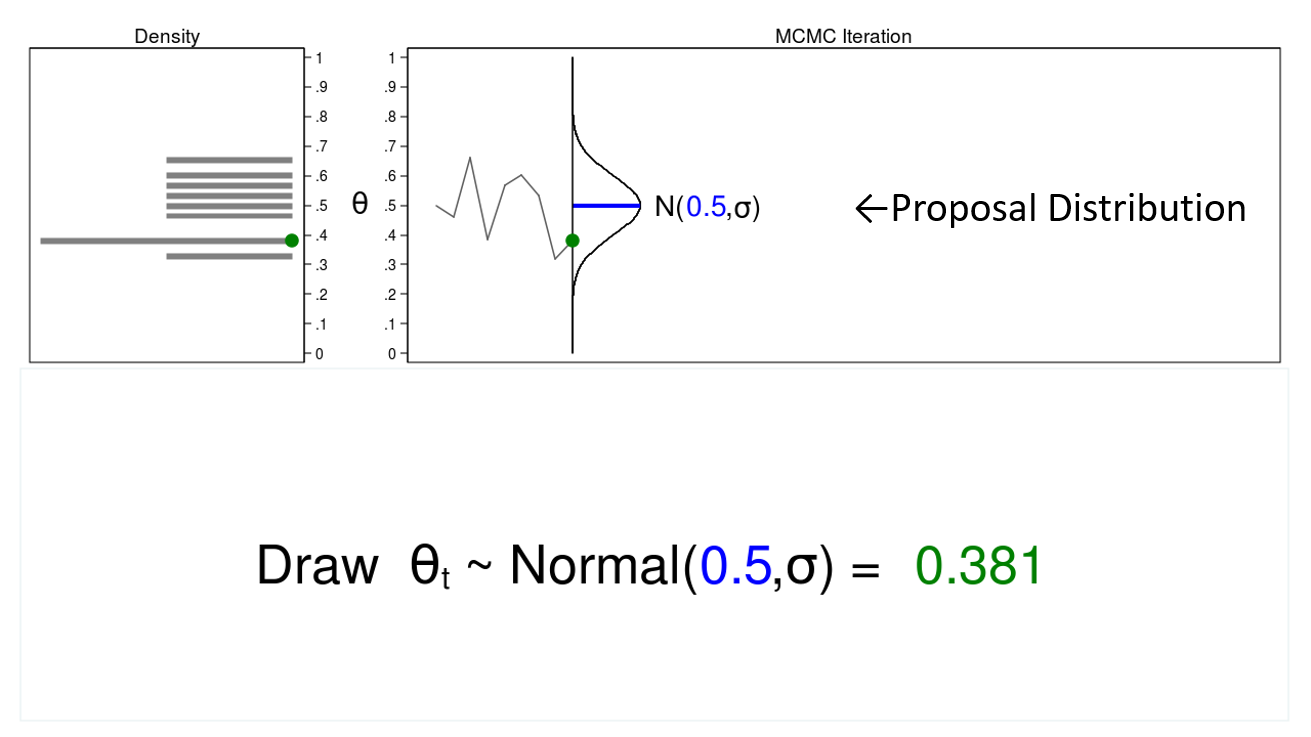
On this instance, I’ll generate a sequence of random numbers from a traditional distribution with a imply of 0.5 and a few arbitrary variance, (sigma). The traditional distribution known as the proposal distribution.
The graph on the highest proper known as a hint plot, and it shows the values of (theta) within the order by which they’re drawn. It additionally shows the proposal distribution rotated clockwise 90 levels, and I’ll shift it to the precise every time I draw a price of theta. The inexperienced level within the hint plot reveals the present worth of (theta).
The density plot on the highest left is a histogram of the pattern that’s rotated counterclockwise 90 levels. I’ve rotated the axes in order that the (theta) axes for each graphs are parallel. Once more, the inexperienced level within the density plot reveals the present worth of (theta).
Let’s draw 10,000 random values of (theta) to see how this course of works.
Animation 1: A Monte Carlo experiment
Animation 1 illustrates a number of essential options. First, the proposal distribution doesn’t change from one iteration to the subsequent. Second, the density plot appears to be like increasingly just like the proposal distribution because the pattern measurement will increase. And third, the hint plot is stationary—the sample of variation appears to be like the identical over all iterations.
Our Monte Carlo simulation generated a pattern that appears very similar to the proposal distribution, and generally that’s all we’d like. However we would require extra instruments to generate a pattern from our posterior distribution.
Markov chain Monte Carlo strategies
A Markov chain is a sequence of numbers the place every quantity depends on the earlier quantity within the sequence. For instance, we might draw values of (theta) from a traditional proposal distribution with a imply equal to the earlier worth of theta.
Determine 2 reveals a hint plot and a density plot the place the present worth of (theta) ((theta_t = 0.530)) was drawn from a proposal distribution with a imply equal to the earlier worth of (theta) ((theta_{t-1} = 0.712)).
Determine 2: A draw from a MCMC experiment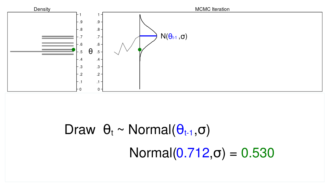
Determine 3 reveals the hint plot and density plot for the subsequent iteration within the sequence. The imply of the proposal density is now (theta_{t-1} = 0.530), and now we have drawn the random quantity ((theta_t = 0.411)) from this new proposal distribution.
Determine 3: The subsequent iteration of the MCMC experiment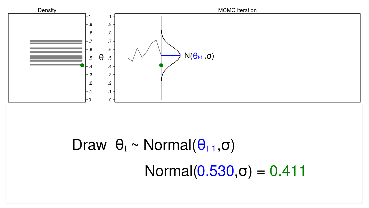
Let’s draw 10,000 random values of (theta) utilizing MCMC to see how this course of works.
Animation 2: A MCMC experiment
Animation 2 reveals two variations between a Monte Carlo experiment and a MCMC experiment. First, the proposal distribution is altering with every iteration. This creates a hint plot with a “random stroll” sample: the variability isn’t the identical over all iterations. Second, the ensuing density plot doesn’t appear like the proposal distribution or another helpful distribution. It actually doesn’t appear like a posterior distribution.
The rationale MCMC alone did not generate a pattern from the posterior distribution is that we haven’t included any details about the
posterior distribution into the method of producing the pattern. We might enhance our pattern by conserving proposed values of (theta) which might be extra doubtless beneath the posterior distribution and discarding values which might be much less doubtless.
However the apparent issue with accepting and rejecting proposed values of (theta) based mostly on the posterior distribution is that we often don’t know the practical type of the posterior distribution. If we knew the practical type, we might calculate chances instantly with out producing a random pattern. So how can we settle for or reject proposed values of (theta) with out realizing the practical type? One reply is the M–H algorithm!
MCMC and the M–H algorithm
The M–H algorithm can be utilized to determine which proposed values of (theta) to just accept or reject even after we don’t know the practical type of the posterior distribution. Let’s break the algorithm into steps and stroll via a number of iterations to see the way it works.
Determine 4: MCMC with the M–H algorithm: Iteration 1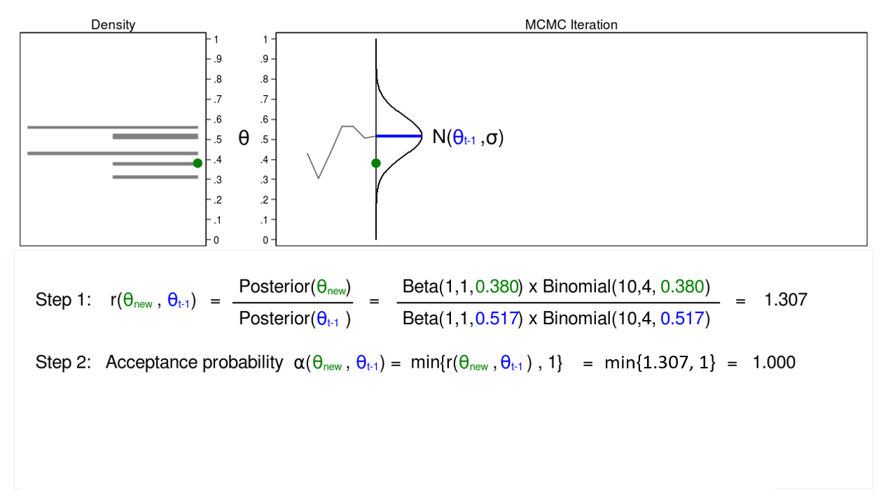
Determine 4 reveals a hint plot and a density plot for a proposal distribution with imply equal to ((theta_{t-1} = 0.0.517)). We’ve drawn a proposed worth of (theta), which is ((theta_mathrm{new} = 0.380)). I’m referring to (theta_mathrm{new}) as “new” as a result of I haven’t determined whether or not to just accept or reject it but.
We start the M–H algorithm with step 1 by calculating the ratio
[
r(theta_mathrm{new},theta_{t-1}) = frac{mathrm{Posterior}(theta_mathrm{new})}{mathrm{Posterior}(theta_{t-1})}
]
We don’t know the practical type of the posterior distribution, however on this instance, we will substitute the product of the prior distribution and the probability perform. The calculation of this ratio isn’t all the time this simple, however we’re attempting to maintain issues easy.
Step 1 in determine 4 reveals that the ratio of the posterior chances for ((theta_mathrm{new} = 0.380)) and ((theta_{t-1} = 0.0.517)) equals 1.307. In step 2, we calculate the settle for likelihood (alpha(theta_mathrm{new},theta_{t-1})), which is solely the minimal of the ratio (r(theta_mathrm{new},theta_{t-1})) and 1. Step 2 is important as a result of chances should fall between 0 and 1.
The acceptance likelihood equals 1, so we settle for ((theta_mathrm{new} = 0.380)), and the imply of our proposal distribution turns into 0.380 within the subsequent iteration.
Determine 5: MCMC with the M–H algorithm: Iteration 2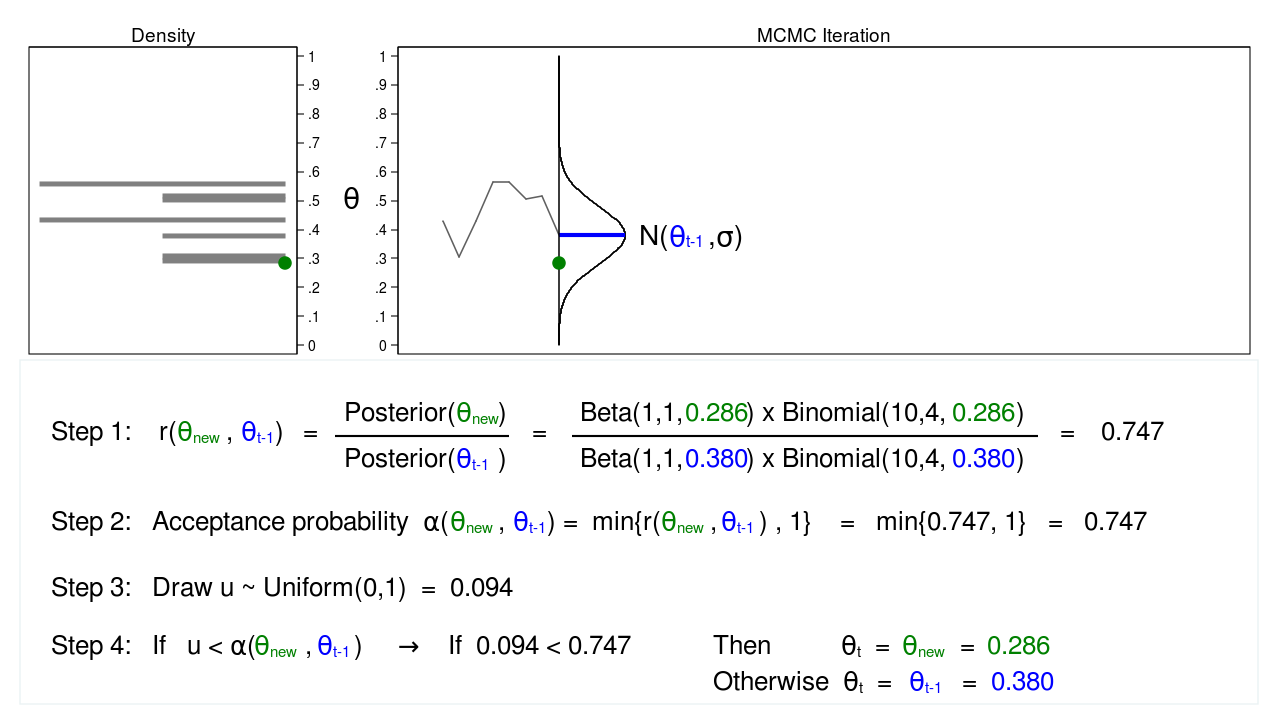
Determine 5 reveals the subsequent iteration the place ((theta_mathrm{new} = 0.286)) has been drawn from our proposal distribution with imply ((theta_{t-1} = 0.380)). The ratio, (r(theta_mathrm{new},theta_{t-1})), calculated in step 1, equals 0.747, which is lower than 1. The acceptance likelihood, (alpha(theta_mathrm{new},theta_{t-1})), calculated in step 2, equals 0.747.
We don’t routinely reject (theta_mathrm{new}) simply because the acceptance likelihood is lower than 1. As an alternative, we draw a random quantity, (u), from a (mathrm{Uniform}(0,1)) distribution in step 3. If (u) is lower than the acceptance likelihood, we settle for the proposed worth of (theta_mathrm{new}). In any other case, we reject (theta_mathrm{new}) and preserve (theta_{t-1}).
Right here (u=0.094) is lower than the acceptance likelihood (0.747), so we are going to settle for ((theta_mathrm{new} = 0.286)). I’ve displayed (theta_mathrm{new}) and 0.286 in inexperienced to point that they’ve been accepted.
Determine 6: MCMC with the M–H algorithm: Iteration 3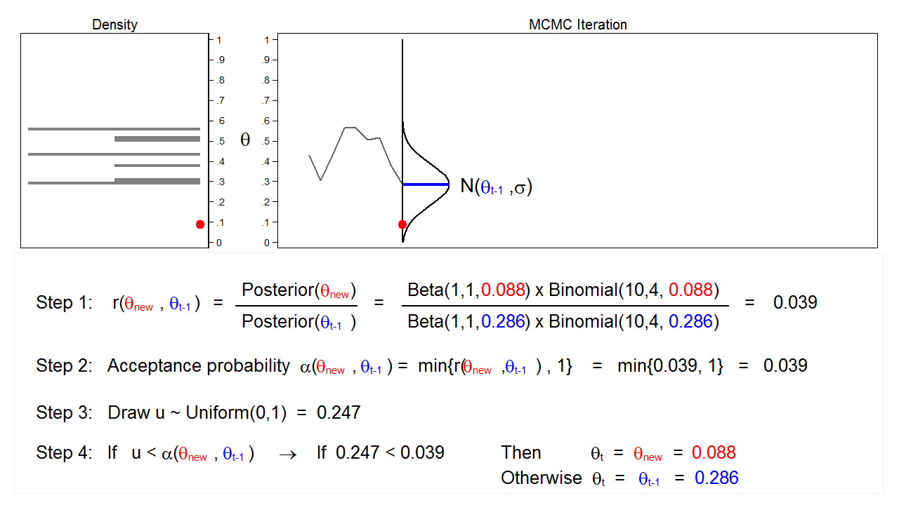
Determine 6 reveals the subsequent iteration the place ((theta_mathrm{new} = 0.088)) has been drawn from our proposal distribution with imply ((theta_{t-1} = 0.286)). The ratio, (r(theta_mathrm{new},theta_{t-1})), calculated in step 1, equals 0.039, which is lower than 1. The acceptance likelihood, (alpha(theta_mathrm{new},theta_{t-1})), calculated in step 2, equals 0.039. The worth of (u), calculated in step 3, is 0.247, which is bigger than the acceptance likelihood. So we reject (theta_mathrm{new}=0.088) and preserve (theta_{t-1} = 0.286) in step 4.
Let’s draw 10,000 random values of (theta) utilizing MCMC with the M–H algorithm to see how this course of works.
Animation 3: MCMC with the M–H algorithm
Animation 3 illustrates a number of issues. First, the proposal distribution modifications with most iterations. Word that proposed values of (theta_mathrm{new}) are displayed in inexperienced if they’re accepted and crimson if they’re rejected. Second, the hint plot doesn’t exhibit the random stroll sample we noticed utilizing MCMC alone. The variation is analogous throughout all iterations, And third, the density plot appears to be like like a helpful distribution.
Let’s rotate the ensuing density plot and take a better look.
Determine 7: A pattern from the posterior distribution generated with MCMC with the M–H algorithm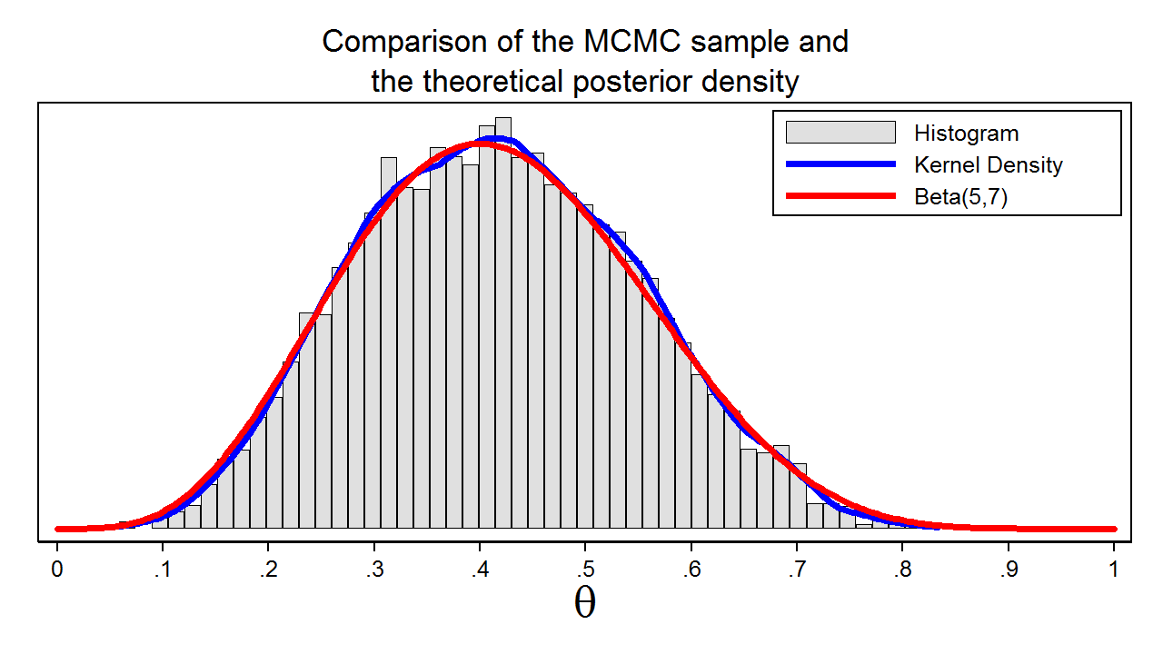
Determine 7 reveals a histogram of the pattern that we generated utilizing MCMC with the M–H algorithm. On this instance, we all know that the posterior distribution is a beta distribution with parameters 5 and seven. The crimson line reveals the analytical posterior distribution, and the blue line is a kernel density plot for our pattern. The kernel density plot is kind of much like the Beta(5,7) distribution, which means that our pattern is an efficient approximation to the theoretical posterior distribution.
We might then use our pattern to calculate the imply or median of the posterior distribution, a 95% credible interval, or the likelihood that (theta) falls inside an arbitrary interval.
MCMC and the M–H algorithm in Stata
Let’s return to our coin toss instance utilizing bayesmh.
We specified a beta distribution with parameters 1 and 1 together with a binomial probability.
Instance 1: Utilizing bayesmh with a Beta(1,1) prior
. bayesmh heads, probability(dbernoulli({theta})) prior({theta}, beta(1,1))

Burn-in ...
Simulation ...

Mannequin abstract
------------------------------------------------------------------------------
Chance:
  heads ~ bernoulli({theta})

Prior:
  {theta} ~ beta(1,1)
------------------------------------------------------------------------------

Bayesian Bernoulli mannequin                         MCMC iterations  =     12,500
Random-walk Metropolis-Hastings sampling         Burn-in          =      2,500
                                                 MCMC pattern measurement =     10,000
                                                 Variety of obs    =         10
                                                 Acceptance charge  =      .4454
Log marginal probability = -7.7989401             Effectivity       =      .2391

------------------------------------------------------------------------------
             |                                                Equal-tailed
             |      Imply   Std. Dev.     MCSE     Median  [95% Cred. Interval]
-------------+----------------------------------------------------------------
       theta |  .4132299   .1370017   .002802   .4101121    .159595   .6818718
------------------------------------------------------------------------------
The output header tells us that bayesmh ran 12,500 MCMC iterations. “Burn-in” tells us that 2,500 of these iterations had been discarded to scale back the affect of the random beginning worth of the chain. The subsequent line within the output tells us that the ultimate MCMC pattern measurement is 10,000, and the subsequent line tells us that there have been 10 observations in our dataset. The acceptance charge is the proportion of proposed values of (theta) that had been included in our remaining MCMC pattern. I’ll refer you to the Stata Bayesian Evaluation Reference Handbook for a definition of effectivity, however excessive effectivity signifies low autocorrelation, and low effectivity signifies excessive autocorrelation. The Monte Carlo normal error (MCSE), proven within the coefficient desk, is an approximation of the error in estimating the true posterior imply.
Checking convergence of the chain
The time period “convergence” has a unique that means within the context of MCMC than within the context of most probability. Algorithms used for optimum probability estimation iterate till they converge to a most. MCMC chains don’t iterate till an optimum worth is recognized. The chain merely iterates till the specified pattern measurement is reached, after which the algorithm stops. The truth that the chain stops operating doesn’t point out that an optimum pattern from the posterior distribution has been generated. We should look at the pattern to examine for issues. We will look at the pattern graphically utilizing bayesgraph diagnostics.
. bayesgraph diagnostics {theta}
Determine 8: Diagnostic plots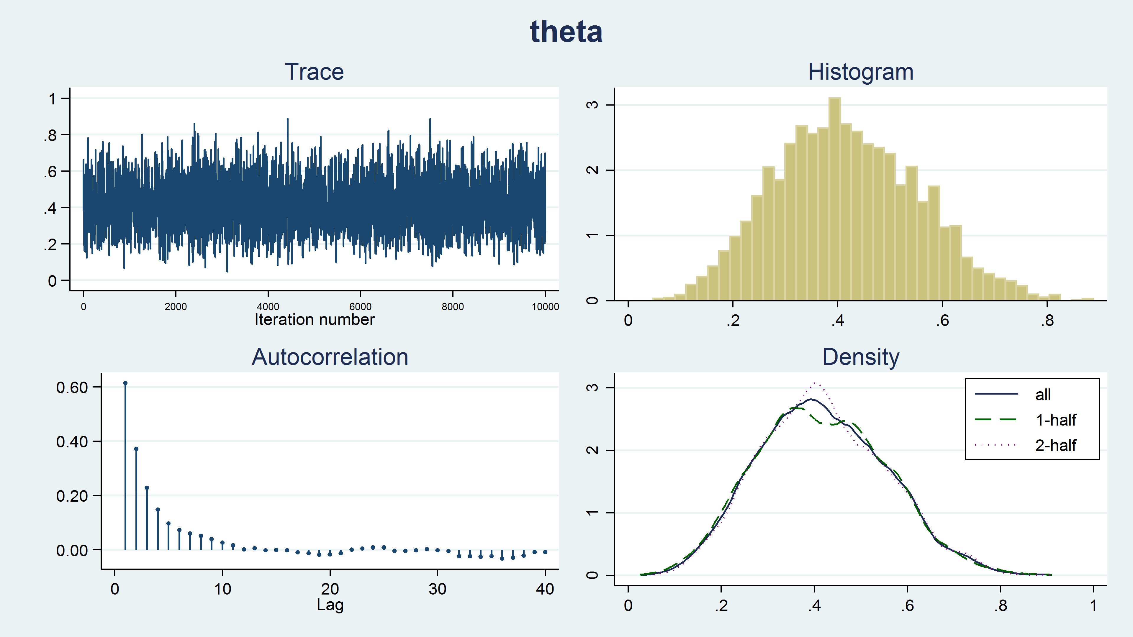
Determine 8 reveals a diagnostic graph that accommodates a hint plot, a histogram and density plots for our MCMC pattern, and a correlegram. The hint plot has a stationary sample, which is what we want to see. The random stroll sample proven in animation 2 signifies issues with the chain. The histogram doesn’t have any uncommon options similar to a number of modes. The kernel density plots for the complete pattern, the primary half of the chain, and the final half of the chain all look comparable and don’t present any unusual options similar to totally different densities for the primary and final half of the chain. Producing the pattern utilizing a Markov chain results in autocorrelation within the pattern, however the autocorrelation decreases shortly for bigger lag values. None of those plots point out any issues with our pattern.
Abstract
This weblog submit launched the concept behind MCMC utilizing the M–H algorithm. Word that I’ve omitted some particulars and ignored some assumptions in order that we might preserve issues easy and develop our instinct. Stata’s bayesmh command really implements a way more subtle algorithm referred to as adaptive MCMC with the M–H algorithm. However the fundamental thought is identical, and I hope I’ve impressed you to attempt it out.
You’ll be able to view a video of this subject on the Stata Youtube Channel right here:
Introduction to Bayesian Statistics, half 2: MCMC and the Metropolis Hastings algorithm