

A loss operate is what guides a mannequin throughout coaching, translating predictions right into a sign it could actually enhance on. However not all losses behave the identical—some amplify giant errors, others keep secure in noisy settings, and every selection subtly shapes how studying unfolds.
Trendy libraries add one other layer with discount modes and scaling results that affect optimization. On this article, we break down the foremost loss households and the way to decide on the suitable one on your job.
Mathematical Foundations of Loss Features
In supervised studying, the target is often to attenuate the empirical threat,
(typically with elective pattern weights and regularization).
the place ℓ is the loss operate, fθ(xi) is the mannequin prediction, and yi is the true goal. In apply, this goal can also embody pattern weights and regularization phrases. Most machine studying frameworks comply with this formulation by computing per-example losses after which making use of a discount corresponding to imply, sum, or none.
When discussing mathematical properties, it is very important state the variable with respect to which the loss is analyzed. Many loss features are convex within the prediction or logit for a set label, though the general coaching goal is normally non-convex in neural community parameters. Necessary properties embody convexity, differentiability, robustness to outliers, and scale sensitivity. Frequent implementation of pitfalls contains complicated logits with chances and utilizing a discount that doesn’t match the meant mathematical definition.
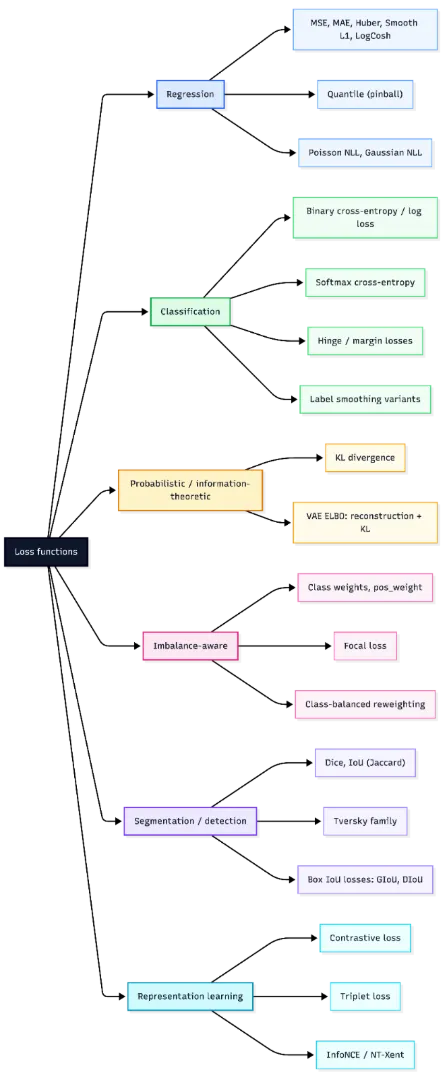
Regression Losses
Imply Squared Error
Imply Squared Error, or MSE, is without doubt one of the most generally used loss features for regression. It’s outlined as the typical of the squared variations between predicted values and true targets:
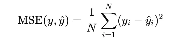
As a result of the error time period is squared, giant residuals are penalized extra closely than small ones. This makes MSE helpful when giant prediction errors needs to be strongly discouraged. It’s convex within the prediction and differentiable all over the place, which makes optimization easy. Nonetheless, it’s delicate to outliers, since a single excessive residual can strongly have an effect on the loss.
import numpy as np
import matplotlib.pyplot as plt

y_true = np.array([3.0, -0.5, 2.0, 7.0])
y_pred = np.array([2.5, 0.0, 2.0, 8.0])

mse = np.imply((y_true - y_pred) ** 2)
print("MSE:", mse)
Imply Absolute Error
Imply Absolute Error, or MAE, measures the typical absolute distinction between predictions and targets:
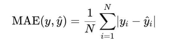
Not like MSE, MAE penalizes errors linearly fairly than quadratically. In consequence, it’s extra sturdy to outliers. MAE is convex within the prediction, however it isn’t differentiable at zero residual, so optimization usually makes use of subgradients at that time.
import numpy as np

y_true = np.array([3.0, -0.5, 2.0, 7.0])
y_pred = np.array([2.5, 0.0, 2.0, 8.0])

mae = np.imply(np.abs(y_true - y_pred))

print("MAE:", mae)
Huber Loss
Huber loss combines the strengths of MSE and MAE by behaving quadratically for small errors and linearly for big ones. For a threshold δ>0, it’s outlined as:
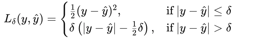
This makes Huber loss a sensible choice when the information are largely effectively behaved however might include occasional outliers.
import numpy as np

y_true = np.array([3.0, -0.5, 2.0, 7.0])
y_pred = np.array([2.5, 0.0, 2.0, 8.0])

error = y_pred - y_true
delta = 1.0

huber = np.imply(
    np.the place(
        np.abs(error) <= delta,
        0.5 * error**2,
        delta * (np.abs(error) - 0.5 * delta)
    )
)

print("Huber Loss:", huber)
Easy L1 Loss
Easy L1 loss is carefully associated to Huber loss and is often utilized in deep studying, particularly in object detection and regression heads. It transitions from a squared penalty close to zero to an absolute penalty past a threshold. It’s differentiable all over the place and fewer delicate to outliers than MSE.
import torch
import torch.nn.purposeful as F

y_true = torch.tensor([3.0, -0.5, 2.0, 7.0])
y_pred = torch.tensor([2.5, 0.0, 2.0, 8.0])

smooth_l1 = F.smooth_l1_loss(y_pred, y_true, beta=1.0)

print("Easy L1 Loss:", smooth_l1.merchandise())
Log-Cosh Loss
Log-cosh loss is a clean different to MAE and is outlined as
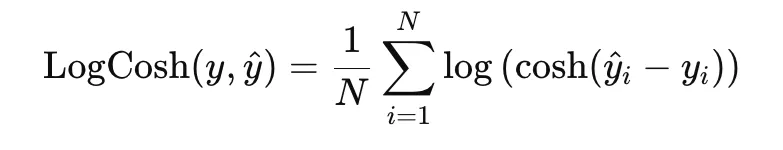
Close to zero residuals, it behaves like squared loss, whereas for big residuals it grows nearly linearly. This provides it an excellent stability between clean optimization and robustness to outliers.
import numpy as np

y_true = np.array([3.0, -0.5, 2.0, 7.0])
y_pred = np.array([2.5, 0.0, 2.0, 8.0])

error = y_pred - y_true

logcosh = np.imply(np.log(np.cosh(error)))

print("Log-Cosh Loss:", logcosh)
Quantile Loss
Quantile loss, additionally referred to as pinball loss, is used when the aim is to estimate a conditional quantile fairly than a conditional imply. For a quantile stage τ∈(0,1) and residual u=y−y^ it’s outlined as
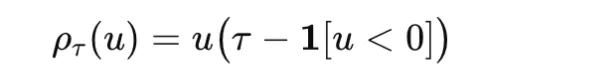
It penalizes overestimation and underestimation asymmetrically, making it helpful in forecasting and uncertainty estimation.
import numpy as np

y_true = np.array([3.0, -0.5, 2.0, 7.0])
y_pred = np.array([2.5, 0.0, 2.0, 8.0])

tau = 0.8

u = y_true - y_pred

quantile_loss = np.imply(np.the place(u >= 0, tau * u, (tau - 1) * u))

print("Quantile Loss:", quantile_loss)
import numpy as np

y_true = np.array([3.0, -0.5, 2.0, 7.0])
y_pred = np.array([2.5, 0.0, 2.0, 8.0])

tau = 0.8

u = y_true - y_pred

quantile_loss = np.imply(np.the place(u >= 0, tau * u, (tau - 1) * u))

print("Quantile Loss:", quantile_loss)
MAPE
Imply Absolute Proportion Error, or MAPE, measures relative error and is outlined as
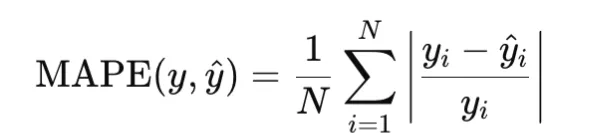
It’s helpful when relative error issues greater than absolute error, but it surely turns into unstable when goal values are zero or very near zero.
import numpy as np

y_true = np.array([100.0, 200.0, 300.0])
y_pred = np.array([90.0, 210.0, 290.0])

mape = np.imply(np.abs((y_true - y_pred) / y_true))

print("MAPE:", mape)
MSLE
Imply Squared Logarithmic Error, or MSLE, is outlined as
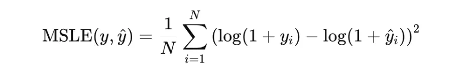
It’s helpful when relative variations matter and the targets are nonnegative.
import numpy as np

y_true = np.array([100.0, 200.0, 300.0])
y_pred = np.array([90.0, 210.0, 290.0])

msle = np.imply((np.log1p(y_true) - np.log1p(y_pred)) ** 2)

print("MSLE:", msle)
Poisson Destructive Log-Probability
Poisson detrimental log-likelihood is used for rely knowledge. For a price parameter λ>0, it’s usually written as
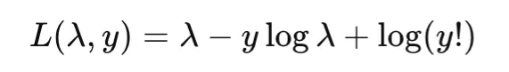
In apply, the fixed time period could also be omitted. This loss is acceptable when targets symbolize counts generated from a Poisson course of.
import numpy as np

y_true = np.array([2.0, 0.0, 4.0])
lam = np.array([1.5, 0.5, 3.0])

poisson_nll = np.imply(lam - y_true * np.log(lam))

print("Poisson NLL:", poisson_nll)
Gaussian Destructive Log-Probability
Gaussian detrimental log-likelihood permits the mannequin to foretell each the imply and the variance of the goal distribution. A typical type is
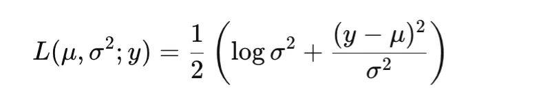
That is helpful for heteroscedastic regression, the place the noise stage varies throughout inputs.
import numpy as np

y_true = np.array([0.0, 1.0])
mu = np.array([0.0, 1.5])
var = np.array([1.0, 0.25])

gaussian_nll = np.imply(0.5 * (np.log(var) + (y_true - mu) ** 2 / var))

print("Gaussian NLL:", gaussian_nll)
Classification and Probabilistic Losses
Binary Cross-Entropy and Log Loss
Binary cross-entropy, or BCE, is used for binary classification. It compares a Bernoulli label y∈{0,1} with a predicted chance p∈(0,1):
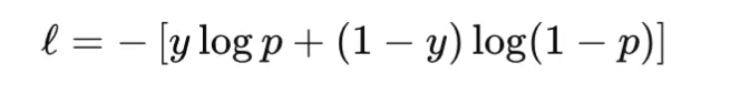
In apply, many libraries want logits fairly than chances and compute the loss in a numerically secure approach. This avoids instability brought on by making use of sigmoid individually earlier than the logarithm. BCE is convex within the logit for a set label and differentiable, however it isn’t sturdy to label noise as a result of confidently improper predictions can produce very giant loss values. It’s broadly used for binary classification, and in multi-label classification it’s utilized independently to every label. A typical pitfall is complicated chances with logits, which might silently degrade coaching.
import torch

logits = torch.tensor([2.0, -1.0, 0.0])
y_true = torch.tensor([1.0, 0.0, 1.0])

bce = torch.nn.BCEWithLogitsLoss()
loss = bce(logits, y_true)

print("BCEWithLogitsLoss:", loss.merchandise())
Softmax Cross-Entropy for Multiclass Classification
Softmax cross-entropy is the usual loss for multiclass classification. For a category index y and logits vector z, it combines the softmax transformation with cross-entropy loss:
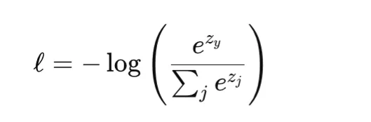
This loss is convex within the logits and differentiable. Like BCE, it could actually closely penalize assured improper predictions and isn’t inherently sturdy to label noise. It’s generally utilized in commonplace multiclass classification and likewise in pixelwise classification duties corresponding to semantic segmentation. One necessary implementation element is that many libraries, together with PyTorch, anticipate integer class indices fairly than one-hot targets until soft-label variants are explicitly used.
import torch
import torch.nn.purposeful as F

logits = torch.tensor([
    [2.0, 0.5, -1.0],
    [0.0, 1.0, 0.0]
], dtype=torch.float32)

y_true = torch.tensor([0, 2], dtype=torch.lengthy)

loss = F.cross_entropy(logits, y_true)

print("CrossEntropyLoss:", loss.merchandise())
Label Smoothing Variant
Label smoothing is a regularized type of cross-entropy during which a one-hot goal is changed by a softened goal distribution. As a substitute of assigning full chance mass to the proper class, a small portion is distributed throughout the remaining courses. This discourages overconfident predictions and might enhance calibration.
The tactic stays differentiable and infrequently improves generalization, particularly in large-scale classification. Nonetheless, an excessive amount of smoothing could make the targets overly ambiguous and result in underfitting.
import torch
import torch.nn.purposeful as F

logits = torch.tensor([
    [2.0, 0.5, -1.0],
    [0.0, 1.0, 0.0]
], dtype=torch.float32)

y_true = torch.tensor([0, 2], dtype=torch.lengthy)

loss = F.cross_entropy(logits, y_true, label_smoothing=0.1)

print("CrossEntropyLoss with label smoothing:", loss.merchandise())
Margin Losses: Hinge Loss
Hinge loss is a basic margin-based loss utilized in help vector machines. For binary classification with label y∈{−1,+1} and rating s, it’s outlined as
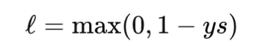
Hinge loss is convex within the rating however not differentiable on the margin boundary. It produces zero loss for examples which might be appropriately categorised with adequate margin, which results in sparse gradients. Not like cross-entropy, hinge loss shouldn’t be probabilistic and doesn’t straight present calibrated chances. It’s helpful when a max-margin property is desired.
import numpy as np

y_true = np.array([1.0, -1.0, 1.0])
scores = np.array([0.2, 0.4, 1.2])

hinge_loss = np.imply(np.most(0, 1 - y_true * scores))

print("Hinge Loss:", hinge_loss)
KL Divergence
Kullback-Leibler divergence compares two chance distributions P and Q:
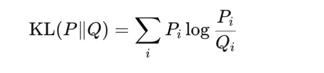
It’s nonnegative and turns into zero solely when the 2 distributions are similar. KL divergence shouldn’t be symmetric, so it isn’t a real metric. It’s broadly utilized in information distillation, variational inference, and regularization of realized distributions towards a previous. In apply, PyTorch expects the enter distribution in log-probability type, and utilizing the improper discount can change the reported worth. Specifically, batchmean matches the mathematical KL definition extra carefully than imply.
import torch
import torch.nn.purposeful as F

P = torch.tensor([[0.7, 0.2, 0.1]], dtype=torch.float32)
Q = torch.tensor([[0.6, 0.3, 0.1]], dtype=torch.float32)

kl_batchmean = F.kl_div(Q.log(), P, discount="batchmean")

print("KL Divergence (batchmean):", kl_batchmean.merchandise())
KL Divergence Discount Pitfall
A typical implementation problem with KL divergence is the selection of discount. In PyTorch, discount=”imply” scales the consequence otherwise from the true KL expression, whereas discount=”batchmean” higher matches the usual definition.
import torch
import torch.nn.purposeful as F

P = torch.tensor([[0.7, 0.2, 0.1]], dtype=torch.float32)
Q = torch.tensor([[0.6, 0.3, 0.1]], dtype=torch.float32)

kl_batchmean = F.kl_div(Q.log(), P, discount="batchmean")
kl_mean = F.kl_div(Q.log(), P, discount="imply")

print("KL batchmean:", kl_batchmean.merchandise())
print("KL imply:", kl_mean.merchandise())
Variational Autoencoder ELBO
The variational autoencoder, or VAE, is skilled by maximizing the proof decrease certain, generally referred to as the ELBO:
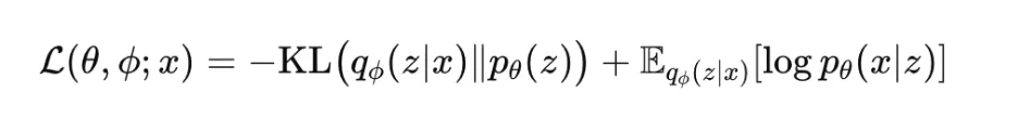
This goal has two components. The reconstruction time period encourages the mannequin to elucidate the information effectively, whereas the KL time period regularizes the approximate posterior towards the prior. The ELBO shouldn’t be convex in neural community parameters, however it’s differentiable underneath the reparameterization trick. It’s broadly utilized in generative modeling and probabilistic illustration studying. In apply, many variants introduce a weight on the KL time period, corresponding to in beta-VAE.
import torch

reconstruction_loss = torch.tensor(12.5)
kl_term = torch.tensor(3.2)

elbo = reconstruction_loss + kl_term

print("VAE-style complete loss:", elbo.merchandise())
Imbalance-Conscious Losses
Class Weights
Class weighting is a typical technique for dealing with imbalanced datasets. As a substitute of treating all courses equally, increased loss weight is assigned to minority courses in order that their errors contribute extra strongly throughout coaching. In multiclass classification, weighted cross-entropy is usually used:
the place wy is the load for the true class. This method is easy and efficient when class frequencies differ considerably. Nonetheless, excessively giant weights could make optimization unstable.
import torch
import torch.nn.purposeful as F

logits = torch.tensor([
    [2.0, 0.5, -1.0],
    [0.0, 1.0, 0.0],
    [0.2, -0.1, 1.5]
], dtype=torch.float32)

y_true = torch.tensor([0, 1, 2], dtype=torch.lengthy)
class_weights = torch.tensor([1.0, 2.0, 3.0], dtype=torch.float32)

loss = F.cross_entropy(logits, y_true, weight=class_weights)

print("Weighted Cross-Entropy:", loss.merchandise())
Constructive Class Weight for Binary Loss
For binary or multi-label classification, many libraries present a pos_weight parameter that will increase the contribution of optimistic examples in binary cross-entropy. That is particularly helpful when optimistic labels are uncommon. In PyTorch, BCEWithLogitsLoss helps this straight.
This methodology is usually most well-liked over naive resampling as a result of it preserves all examples whereas adjusting the optimization sign. A typical mistake is to confuse weight and pos_weight, since they have an effect on the loss otherwise.
import torch

logits = torch.tensor([2.0, -1.0, 0.5], dtype=torch.float32)
y_true = torch.tensor([1.0, 0.0, 1.0], dtype=torch.float32)

criterion = torch.nn.BCEWithLogitsLoss(pos_weight=torch.tensor([3.0]))
loss = criterion(logits, y_true)

print("BCEWithLogitsLoss with pos_weight:", loss.merchandise())
Focal Loss
Focal loss is designed to handle class imbalance by down-weighting straightforward examples and focusing coaching on tougher ones. For binary classification, it’s generally written as
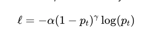
the place pt is the mannequin chance assigned to the true class, α is a class-balancing issue, and γ controls how strongly straightforward examples are down-weighted. When γ=0, focal loss reduces to unusual cross-entropy.
Focal loss is broadly utilized in dense object detection and extremely imbalanced classification issues. Its predominant hyperparameters are α and γ, each of which might considerably have an effect on coaching habits.
import torch
import torch.nn.purposeful as F

logits = torch.tensor([2.0, -1.0, 0.5], dtype=torch.float32)
y_true = torch.tensor([1.0, 0.0, 1.0], dtype=torch.float32)

bce = F.binary_cross_entropy_with_logits(logits, y_true, discount="none")

probs = torch.sigmoid(logits)
pt = torch.the place(y_true == 1, probs, 1 - probs)

alpha = 0.25
gamma = 2.0

focal_loss = (alpha * (1 - pt) ** gamma * bce).imply()

print("Focal Loss:", focal_loss.merchandise())
Class-Balanced Reweighting
Class-balanced reweighting improves on easy inverse-frequency weighting through the use of the efficient variety of samples fairly than uncooked counts. A typical system for the category weight is
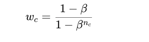
the place nc is the variety of samples in school c and β is a parameter near 1. This provides smoother and infrequently extra secure reweighting than direct inverse counts.
This methodology is helpful when class imbalance is extreme however naive class weights could be too excessive. The primary hyperparameter is β, which determines how strongly uncommon courses are emphasised.
import numpy as np

class_counts = np.array([1000, 100, 10], dtype=np.float64)
beta = 0.999

effective_num = 1.0 - np.energy(beta, class_counts)
class_weights = (1.0 - beta) / effective_num

class_weights = class_weights / class_weights.sum() * len(class_counts)

print("Class-Balanced Weights:", class_weights)
Segmentation and Detection Losses
Cube Loss
Cube loss is broadly utilized in picture segmentation, particularly when the goal area is small relative to the background. It’s primarily based on the Cube coefficient, which measures overlap between the expected masks and the ground-truth masks:
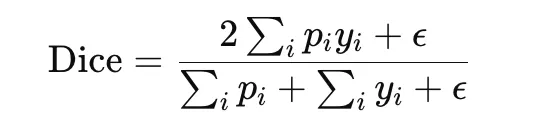
The corresponding loss is
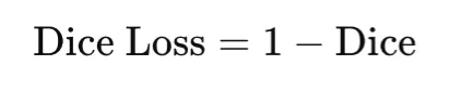
Cube loss straight optimizes overlap and is subsequently effectively suited to imbalanced segmentation duties. It’s differentiable when smooth predictions are used, however it may be delicate to small denominators, so a smoothing fixed ϵ is normally added.
import torch

y_true = torch.tensor([1, 1, 0, 0], dtype=torch.float32)
y_pred = torch.tensor([0.9, 0.8, 0.2, 0.1], dtype=torch.float32)

eps = 1e-6

intersection = torch.sum(y_pred * y_true)
cube = (2 * intersection + eps) / (torch.sum(y_pred) + torch.sum(y_true) + eps)

dice_loss = 1 - cube

print("Cube Loss:", dice_loss.merchandise())
IoU Loss
Intersection over Union, or IoU, additionally referred to as Jaccard index, is one other overlap-based measure generally utilized in segmentation and detection. It’s outlined as
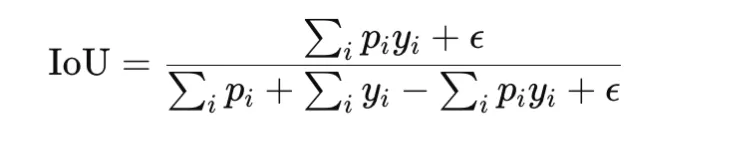
The loss type is
IoU loss is stricter than Cube loss as a result of it penalizes disagreement extra strongly. It’s helpful when correct area overlap is the primary goal. As with Cube loss, a small fixed is added for stability.
import torch

y_true = torch.tensor([1, 1, 0, 0], dtype=torch.float32)
y_pred = torch.tensor([0.9, 0.8, 0.2, 0.1], dtype=torch.float32)

eps = 1e-6

intersection = torch.sum(y_pred * y_true)
union = torch.sum(y_pred) + torch.sum(y_true) - intersection

iou = (intersection + eps) / (union + eps)
iou_loss = 1 - iou

print("IoU Loss:", iou_loss.merchandise())
Tversky Loss
Tversky loss generalizes Cube and IoU type overlap losses by weighting false positives and false negatives otherwise. The Tversky index is
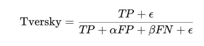
and the loss is
This makes it particularly helpful in extremely imbalanced segmentation issues, corresponding to medical imaging, the place lacking a optimistic area could also be a lot worse than together with further background. The selection of α and β controls this tradeoff.
import torch

y_true = torch.tensor([1, 1, 0, 0], dtype=torch.float32)
y_pred = torch.tensor([0.9, 0.8, 0.2, 0.1], dtype=torch.float32)

eps = 1e-6
alpha = 0.3
beta = 0.7

tp = torch.sum(y_pred * y_true)
fp = torch.sum(y_pred * (1 - y_true))
fn = torch.sum((1 - y_pred) * y_true)

tversky = (tp + eps) / (tp + alpha * fp + beta * fn + eps)
tversky_loss = 1 - tversky

print("Tversky Loss:", tversky_loss.merchandise())
Generalized IoU Loss
Generalized IoU, or GIoU, is an extension of IoU designed for bounding-box regression in object detection. Customary IoU turns into zero when two bins don’t overlap, which provides no helpful gradient. GIoU addresses this by incorporating the smallest enclosing field CCC:
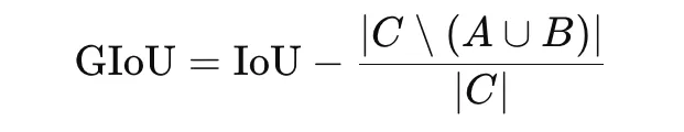
The loss is

GIoU is helpful as a result of it nonetheless gives a coaching sign even when predicted and true bins don’t overlap.
import torch

def box_area(field):
    return max(0.0, field[2] - field[0]) * max(0.0, field[3] - field[1])

def intersection_area(box1, box2):
    x1 = max(box1[0], box2[0])
    y1 = max(box1[1], box2[1])
    x2 = min(box1[2], box2[2])
    y2 = min(box1[3], box2[3])
    return max(0.0, x2 - x1) * max(0.0, y2 - y1)

pred_box = [1.0, 1.0, 3.0, 3.0]
true_box = [2.0, 2.0, 4.0, 4.0]

inter = intersection_area(pred_box, true_box)
area_pred = box_area(pred_box)
area_true = box_area(true_box)

union = area_pred + area_true - inter
iou = inter / union

c_box = [
    min(pred_box[0], true_box[0]),
    min(pred_box[1], true_box[1]),
    max(pred_box[2], true_box[2]),
    max(pred_box[3], true_box[3]),
]

area_c = box_area(c_box)
giou = iou - (area_c - union) / area_c

giou_loss = 1 - giou

print("GIoU Loss:", giou_loss)
Distance IoU Loss
Distance IoU, or DIoU, extends IoU by including a penalty primarily based on the gap between field facilities. It’s outlined as
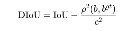
the place ρ2(b,bgt) is the squared distance between the facilities of the expected and ground-truth bins, and c2 is the squared diagonal size of the smallest enclosing field. The loss is

DIoU improves optimization by encouraging each overlap and spatial alignment. It’s generally utilized in bounding-box regression for object detection.
import math

def box_center(field):
    return ((field[0] + field[2]) / 2.0, (field[1] + field[3]) / 2.0)

def intersection_area(box1, box2):
    x1 = max(box1[0], box2[0])
    y1 = max(box1[1], box2[1])
    x2 = min(box1[2], box2[2])
    y2 = min(box1[3], box2[3])
    return max(0.0, x2 - x1) * max(0.0, y2 - y1)

pred_box = [1.0, 1.0, 3.0, 3.0]
true_box = [2.0, 2.0, 4.0, 4.0]

inter = intersection_area(pred_box, true_box)

area_pred = (pred_box[2] - pred_box[0]) * (pred_box[3] - pred_box[1])
area_true = (true_box[2] - true_box[0]) * (true_box[3] - true_box[1])

union = area_pred + area_true - inter
iou = inter / union

cx1, cy1 = box_center(pred_box)
cx2, cy2 = box_center(true_box)

center_dist_sq = (cx1 - cx2) ** 2 + (cy1 - cy2) ** 2

c_x1 = min(pred_box[0], true_box[0])
c_y1 = min(pred_box[1], true_box[1])
c_x2 = max(pred_box[2], true_box[2])
c_y2 = max(pred_box[3], true_box[3])

diag_sq = (c_x2 - c_x1) ** 2 + (c_y2 - c_y1) ** 2

diou = iou - center_dist_sq / diag_sq
diou_loss = 1 - diou

print("DIoU Loss:", diou_loss)
Illustration Studying Losses
Contrastive Loss
Contrastive loss is used to be taught embeddings by bringing comparable samples nearer collectively and pushing dissimilar samples farther aside. It’s generally utilized in Siamese networks. For a pair of embeddings with distance d and label y∈{0,1}, the place y=1 signifies an identical pair, a typical type is
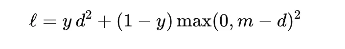
the place m is the margin. This loss encourages comparable pairs to have small distance and dissimilar pairs to be separated by no less than the margin. It’s helpful in face verification, signature matching, and metric studying.
import torch
import torch.nn.purposeful as F

z1 = torch.tensor([[1.0, 2.0]], dtype=torch.float32)
z2 = torch.tensor([[1.5, 2.5]], dtype=torch.float32)

label = torch.tensor([1.0], dtype=torch.float32)  # 1 = comparable, 0 = dissimilar

distance = F.pairwise_distance(z1, z2)

margin = 1.0

contrastive_loss = (
    label * distance.pow(2)
    + (1 - label) * torch.clamp(margin - distance, min=0).pow(2)
)

print("Contrastive Loss:", contrastive_loss.imply().merchandise())
Triplet Loss
Triplet loss extends pairwise studying through the use of three examples: an anchor, a optimistic pattern from the identical class, and a detrimental pattern from a distinct class. The target is to make the anchor nearer to the optimistic than to the detrimental by no less than a margin:
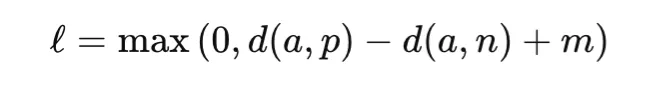
the place d(⋅, ⋅) is a distance operate and m is the margin. Triplet loss is broadly utilized in face recognition, individual re-identification, and retrieval of duties. Its success relies upon strongly on how informative triplets are chosen throughout coaching.
import torch
import torch.nn.purposeful as F

anchor = torch.tensor([[1.0, 2.0]], dtype=torch.float32)
optimistic = torch.tensor([[1.1, 2.1]], dtype=torch.float32)
detrimental = torch.tensor([[3.0, 4.0]], dtype=torch.float32)

margin = 1.0

triplet = torch.nn.TripletMarginLoss(margin=margin, p=2)
loss = triplet(anchor, optimistic, detrimental)

print("Triplet Loss:", loss.merchandise())
InfoNCE and NT-Xent Loss
InfoNCE is a contrastive goal broadly utilized in self-supervised illustration studying. It encourages an anchor embedding to be near its optimistic pair whereas being removed from different samples within the batch, which act as negatives. A normal type is
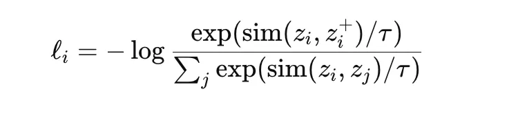
the place sim is a similarity measure corresponding to cosine similarity and τ is a temperature parameter. NT-Xent is a normalized temperature-scaled variant generally utilized in strategies corresponding to SimCLR. These losses are highly effective as a result of they be taught wealthy representations with out guide labels, however they rely strongly on batch composition, augmentation technique, and temperature selection.
import torch
import torch.nn.purposeful as F

z_anchor = torch.tensor([[1.0, 0.0]], dtype=torch.float32)
z_positive = torch.tensor([[0.9, 0.1]], dtype=torch.float32)
z_negative1 = torch.tensor([[0.0, 1.0]], dtype=torch.float32)
z_negative2 = torch.tensor([[-1.0, 0.0]], dtype=torch.float32)

embeddings = torch.cat([z_positive, z_negative1, z_negative2], dim=0)

z_anchor = F.normalize(z_anchor, dim=1)
embeddings = F.normalize(embeddings, dim=1)

similarities = torch.matmul(z_anchor, embeddings.T).squeeze(0)

temperature = 0.1
logits = similarities / temperature

labels = torch.tensor([0], dtype=torch.lengthy)  # optimistic is first

loss = F.cross_entropy(logits.unsqueeze(0), labels)

print("InfoNCE / NT-Xent Loss:", loss.merchandise())
Comparability Desk and Sensible Steerage
The desk beneath summarizes key properties of generally used loss features. Right here, convexity refers to convexity with respect to the mannequin output, corresponding to prediction or logit, for fastened targets, not convexity in neural community parameters. This distinction is necessary as a result of most deep studying targets are non-convex in parameters, even when the loss is convex within the output.
| Loss | Typical Activity | Convex in Output | Differentiable | Sturdy to Outliers | Scale / Models |
|---|---|---|---|---|---|
| MSE | Regression | Sure | Sure | No | Squared goal items |
| MAE | Regression | Sure | No (kink) | Sure | Goal items |
| Huber | Regression | Sure | Sure | Sure (managed by δ) | Goal items |
| Easy L1 | Regression / Detection | Sure | Sure | Sure | Goal items |
| Log-cosh | Regression | Sure | Sure | Reasonable | Goal items |
| Pinball (Quantile) | Regression / Forecast | Sure | No (kink) | Sure | Goal items |
| Poisson NLL | Rely Regression | Sure (λ>0) | Sure | Not major focus | Nats |
| Gaussian NLL | Uncertainty Regression | Sure (imply) | Sure | Not major focus | Nats |
| BCE (logits) | Binary / Multilabel | Sure | Sure | Not relevant | Nats |
| Softmax Cross-Entropy | Multiclass | Sure | Sure | Not relevant | Nats |
| Hinge | Binary / SVM | Sure | No (kink) | Not relevant | Margin items |
| Focal Loss | Imbalanced Classification | Usually No | Sure | Not relevant | Nats |
| KL Divergence | Distillation / Variational | Context-dependent | Sure | Not relevant | Nats |
| Cube Loss | Segmentation | No | Virtually (smooth) | Not major focus | Unitless |
| IoU Loss | Segmentation / Detection | No | Virtually (smooth) | Not major focus | Unitless |
| Tversky Loss | Imbalanced Segmentation | No | Virtually (smooth) | Not major focus | Unitless |
| GIoU | Field Regression | No | Piecewise | Not major focus | Unitless |
| DIoU | Field Regression | No | Piecewise | Not major focus | Unitless |
| Contrastive Loss | Metric Studying | No | Piecewise | Not major focus | Distance items |
| Triplet Loss | Metric Studying | No | Piecewise | Not major focus | Distance items |
| InfoNCE / NT-Xent | Contrastive Studying | No | Sure | Not major focus | Nats |
Conclusion
Loss features outline how fashions measure error and be taught throughout coaching. Totally different duties—regression, classification, segmentation, detection, and illustration studying—require totally different loss varieties. Selecting the best one relies on the issue, knowledge distribution, and error sensitivity. Sensible concerns like numerical stability, gradient scale, discount strategies, and sophistication imbalance additionally matter. Understanding loss features results in higher coaching and extra knowledgeable mannequin design selections.
Often Requested Questions
A. It measures the distinction between predictions and true values, guiding the mannequin to enhance throughout coaching.
A. It relies on the duty, knowledge distribution, and which errors you wish to prioritize or penalize.
A. They have an effect on gradient scale, influencing studying price, stability, and total coaching habits.
Hello, I’m Janvi, a passionate knowledge science fanatic presently working at Analytics Vidhya. My journey into the world of knowledge started with a deep curiosity about how we will extract significant insights from complicated datasets.
Login to proceed studying and revel in expert-curated content material.